SGE DataArtist – User Manual

www.sge-ing.de – Version 1.62.67 (2022-07-24 22:21)

1 Introduction

The SGE DataArtist is a tool to visualize and analyze measurement data. This manual contains information concerning specifically the SGE DataArtist only. The SGE DataArtist is part of the SGE Circus. For help topics regarding general features please refer to the corresponding documentation accessible using the links below.

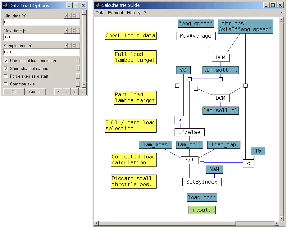
1.1 SGE Circus user manual The SGE Circus documentation makes available general information regarding data loading procedure, input handling, preferences, history and other topics concerning all tools.	1.2 SGE CalcGuide user manual The SGE CalcGuide is a tool to implement calculation routines by creating graphical flow chart diagrams - included with all tools.

1.3 SGE Circus videos (external) Videos and tutorials are available on the internet.

For information regarding the version dependent software changes please refer to the Release notes accessible using the corresponding menu item inside the SGE Circus.

2 Keyboard shortcuts, mouse gestures

Many functions are quickly accessible via keyboard shortcuts. For a list of available keyboard shortcuts, see the list below. In addition, the entries in the menus and context menus as well as the tooltips of the toolbar point to shortcuts.

Data Handling
Ctrl + Shift + o	Add FileSet... Multiple files will be appended to one FileSet.
Alt + Shift + o	Add FileSet quick... Just the files will be asked – the options will be maintained.
Shift + o	Add multiple FileSets... Multiple files will be opened as multiple FileSet comparison overlay.
Ctrl + o	Replace FileSet, Open first FileSet...
Alt + o	Replace FileSet quick... Just the files will be asked – the options will be maintained.
Ctrl + Del	Delete all channel(s) of one or multiple FileSet...
Ctrl + s	Save data...
Ctrl + Shift + s	Save session...
Ctrl + d	Delete data...
Ctrl + c	Copy data to clipboard
Ctrl + v	Paste files from clipboard into present session...
Ctrl + Shift + i	Data info
Ctrl + m	Edit file comment...
Template Handling
Shift + t	Open template...
Shift + s	Save template ...
Main View
+/- Mouse left button drag Ctrl + Mouse Wheel	Zoom in / out
Mouse double click into cursor value table	Center view to cursor
Shift+space	Zoom to cursors (if two cursors are present)
(Ctrl + ) ← → (Ctrl + ) Pageup/down Mouse right button drag Mouse Wheel	Pan left / right Ctrl + Pageup/down pans one axis unit and can be used to pan exactly one cycle if the axis is combustion cycles for indicating measurements.
Ctrl + r Ctrl + F12	Reset axis view to cover entire file(s)
Mouse drag at left/right end of main view	Resize main view to create space for the cursor if these should not overlay the main view.
Ctrl + x	Set x-axis range...
Ctrl + shift + c	Copy window to clipboard..., Print window...
F5	Snapshot all artists
Overview
F6	Toggle overview
Ctrl + F6	Add / remove channel to / from overview
Shift + ← →	Focus section left / right
GPS view
+/- Mouse left button drag Ctrl + Mouse Wheel	Zoom in / out
Ctrl + r Ctrl + F12	Reset axis view to cover entire file(s)
Cursor
Space	Cursor on / off
Ctrl + space	Insert new cursor
Esc	Delete cursor
Shift + 1..9, Mouse click	Set active cursor
Mouse double click into cursor value table	Center view to cursor
Shift+space	Zoom to cursors (if two cursors are present)
← →	Move cursor left / right
Ctrl + Shift + ← →	Move cursor left / right until next value change of selected channel
Ctrl + Shift + Up / Down	Move channel in cursor list
Alt + h	Toggle cursor options “Show hidden channels” and “Show only selected channel”.
Channels
Ins	Add channel(s) to the FileSet that correlates to the selected channel...
Ctrl + Shift + Ins	Add channel(s) to all FileSets. The selected channel dictates the FileSet whose channel list will be presented for channel selection.
Del	Delete channel(s)...
Ctrl + Del	Delete all channel(s) of one or multiple FileSet...
Enter Mouse double click	Channel range set. Common Y axes arrangement.
Ctrl + 0..9	Switch predefined ranges for selected channel (repeatedly)
Ctrl + Shift + 0,ß	Switch predefined ranges for all channels
Ctrl + +/- Ctrl + Drag with right button pressed	Scale selected channel
Ctrl + Up / Down Drag with right button pressed	Move selected channel up / down
Shift + enter	Color channel...
Shift + n	Next color
Ctrl + n	Previous color
Ctrl + h	Hide / show channel
Shift + h	Hide / show all channels sharing the common Y axes of the selected channel
Ctrl + Shift + h	Hide / show all channels sharing the FileSet of the selected channel
Esc	Unselect all channels
Ctrl + Mouse click	Add channel to the common Y axes of the currently selected channel. Show channel if hidden.
a..z0..9_-*	Select channel by uninterrupted typing of its name. Use * as wildcard character.
F2	Rename selected channel...
Ctrl + F2	Rename all channels using replacement patterns...
Ctrl + shift + x Mouse right button drag*	Axis shift of channel(s)... * When multiple FileSets loaded
Ctrl + Shift + Up / Down	Move channel in cursor list
Ctrl + F6	Add / remove channel to / from overview
F3	Select channel... Hide/show all other channels.
F4	Channel configuration utility (manual)...
Shift + F4	Channel styling utility (using patterns)...
Ctrl + f	Channel wizard (filter etc.)...
Ctrl + i	Channel info...
Shift + z	Toggle markers for selected channel or all if none is selected.
Ctrl + Shift + z	Toggle markers +lines for selected channel or all if none is selected.
Tabs
Ctrl + t	Add tab...
Ctrl/Shift + tab	Activate next/previous tab
Marks
Shift + Ins	Add mark...
Shift + Del	Delete mark(s)
Ctrl + Shift + Del	Delete marks by condition...
Shift + i	„Split equally“ mark creation...
Shift + c	„Classification split“ mark creation
Shift + r	„Ramp / step detection“ mark creation
Shift + l	„Logical“ mark creation
Shift + x	Cut / extend marks...
Ctrl + Shift + F4	Configure marks (color, transparency)...
Annotations
Ctrl+a	Toggle visibility of the annotations
Ctrl + Shift + a	Add annotation manually...
Alt + Shift + a	Add annotations from file...
Shift + a	Select annotation...
Enter	Edit selected annotation...
Del	Delete selected annotation...
Undo / Redo
F1	Show manual...
Shift+F1	Show keyboard shortcut manual...
Ctrl + z	Undo (views, marks)
Ctrl + y	Redo (views, marks)

3 Features

The main features of the SGE DataArtist are listed in this introduction. For details please see the following sections.

Data Import

Formats MDF3/4, ASCII, Diadem, FAMOS, Horiba-VTS, IFile, Kistler *.ifi, BLF/ASC CAN files, Excel*, OpenOffice*, MATLAB, Magneti Marelli, MoTeC, 2D-Logger, Get-Logger, Tellert, Keihin (* if Apache OpenOffice or Microsoft Excel is installed)
Data import from MATLAB workspace, function calls, Simulink simulations and DLL output
Automatic synchronization from IFiles to respective MDF measurements. This enables a parallel evaluation of crank angle based indication measurements, e.g. cylinder pressure traces in time based measurements.
Any number of files and FileSets can be loaded and are synchronized automatically.
Separate / common time pattern, down-sampling, time period
Loaded data can be filtered by any logical expression
Powerful data / comment preview during file selection
Definition of any number of calculated channels including features like map interpolation and Simulink systems integration
x/y-plot

Data Export

Formats MDF3/4, ASCII, Excel, OpenOffice, MATLAB, Google Maps/Earth
Channels, time periods selectable
Statistical data

Session

The whole session including data can be stored as file. After re-opening the whole functionality can be used again immediately.
File size is depending on loaded data.

Template

The session-configuration can be stored as a template.
When the template is loaded, the session is reconstructed.
Quick swap between prepared standard-configurations
Minimum file size
LastTemplate allows to reconstruct the last session without previous saving.

History

Undo- / Redo-function for display and mark activities
All dialog have a history and filters to find former inputs quickly.
All dialog offer export and import functionality to load and document inputs.

Display Configuration

Channels can be displayed as Stairs / Lines / Stems / Marker or in s scatter view using a color source channel
Channel scaling manual, predefined, automatic, smart range or mouse driven
Overview-chart, GPS-overview
Automatic down-sampling for visualization of large data volumes
Tabs enable to create multiple views in parallel

Cursor

Any number of Cursors displayable
Configurable appearance (e.g. differences, units)
Cursor difference absolute and/or relative
Channel order can be sorted or adjusted manually
Legend position left or right

Marks

Sections can be marked manually or automatically
Split: Split of sections in n parts
Channel classification: Partition of sections in e.g. constant temperature or engine speed steps
Logical detection: Mark of areas by logical conditions
Ramp detection: Automatic detection of constant phases, ramp measurements, cost down measurements ect.
Import: Mark sections with the help of external data

Annotations

Add annotations to highlight and notice events in the data loaded.

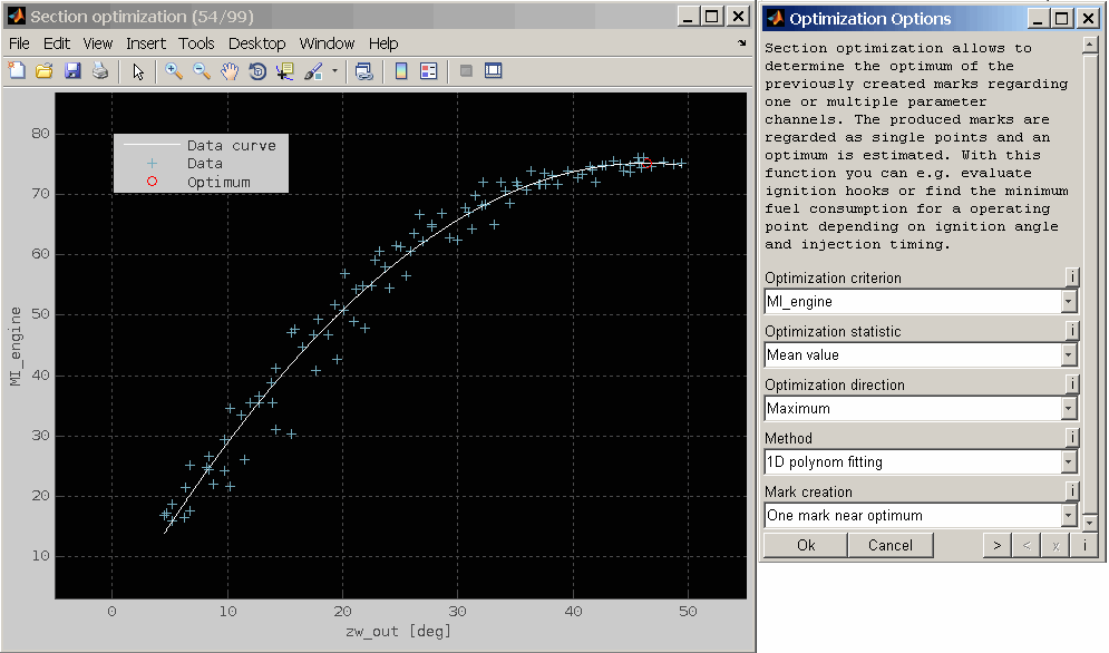
Section Optimization

Automated parameter-optimization graphically guided or fully automated
Criteria: Max, Min, Mean, Std
Direction: Minimum, Maximum
1- and 2-parameter-optimization
Polynomial-, Cubic-, Map fit, Simple selection
Evaluation of ignition sweeps, parameter variation of injection angle, camshaft actuator etc.
Possibility to check and adjust every section manually

Data Processing

Direct access to standard tasks of data processing
- Moving average, digital FIR filter
- Duplicate removal
- Accumulated sums (relative or absolute)
- Polynomial fit
- Exponential fit (e.g. estimation of the terminal value of exhaust gas temperatures)
- Detrend
"Unlimited" possibilities by utilization of calculated channels

Measurement Information

Display of information about loaded FileSets, files, periods and calculated channels
Documentation and Validation
Display and Edit measurement comments (MDF3/4, 2D, Keihin)

Channel Information

Statistic values of the currently visible part of the selected channel and its axis
Min, Max, Mean, Std, Curve fits
Quick determination of gradients, mean values and standard deviations

Graphic Export

Configurable export of the actual screen to the clipboard
Ready formatted for email or office software. Reports made easy.
Axes, fonts, sizes, adjustable. Adding notes, highlights, etc.

Data Exchange

Copying selected channel data to clipboard
Print window

4 Data handling

The data loading procedure is explained in the documentation of the SGE_Circus because as it is common to all tools. We recommend that you read that section first as useful features like sample reduction, logical load conditions, calculated channels are explained there.

→ SGE Circus documentation "Loading data"

4.1 Open / Add / Replace FileSet

When starting the DataArtist you will be immediately asked for files and channels to load. Data is organized in so called FileSets. A FileSet consists of one or more files. In the case of multiple files, the files are automatically sequenced. To be able to recognize the file borders, the channel “FileCnt” can be loaded, which displays them graphically and textually, if the text translation option is active in the cursor (Cursors).

The DataArtist can handle multiple FileSets. So when you already have loaded data and you choose to add another FileSet the data loading procedure is repeated and a second FileSet is created. The channels names are extended with “_F2” for second FileSet. If the second FileSet contains channels that are also loaded in the first FileSet they are put together on common Y axes and colored similarly.

Using drag and drop or pasting files enables to quickly load any number of files. See the following chapter for details.

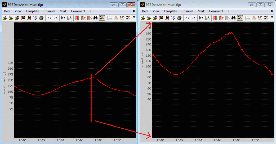
FileSets can be shifted and synchronized. You can simply pick any channel of a FileSet with the right mouse button and drag it horizontally. After releasing the mouse button you can decide whether to shift all channels of this FileSet accordingly. Alternatively you can do a automatic synchronization (see below).

Several modes to add and replace data are supported.

Add FileSet, session, template... (Ctrl + Shift + o)

Add data from one or multiple files. One new FileSet will be created from the data by appending the files sequentially. This way any number of files can be loaded and processed at once.

Because of the appending this mode is not suitable for comparison of the single files. Add multiple FileSets successively or use "Add multiple FileSets" if you want to overlay or compare data from multiple files.

Drag&Drop and Copy/Paste is also available and also session and template files can be opened.
Add FileSet quick... (Ctrl + Shift + o)

Quickly add a new FileSet. Only the files will be asked. The options will be adopted from the actual FileSet which is the one of the selected channel or the first one if no channel is selected. Again multiple files can be selected at once and will be appended to one FileSet sequentially.

Drag&Drop and Copy/Paste is also available and also session and template files can be opened.
Add multiple FileSets... (Shift + o)

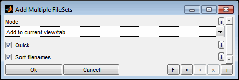
In this mode the single files will not be appended to a single FileSet. Instead individual FileSets will be created. Depending on the mdoe chosen these will be done to create a FileSets comparison overlay or to add separate tabs for the single files.
- Mode
  
  Choose how to handle the file(s) to add.
  - Add to current view/tab
    
    For each file to load a new FileSets inside the current view/tab will be created to obtain and overlay of the single FileSets. Use this mode to compare and overlay multiple files.
  - Create a new tab for each file
    
    For each file to load a new individual Tab will be created. When data is already loaded without a tab existing a new tab will be created first automatically for this data.
- Quick
  
  When selected the options will be asked only once and no options will be asked from the second FileSet. They will be adopted from the existing FileSet.
- Sort filenames
  
  When selected the filenames will be sorted before processing.
Drag&Drop and Copy/Paste is also available and also session and template files can be opened.
Replace FileSet... (Ctrl + o)

Replace the data of the actual FileSet. Channels and options will be asked again. The actual FileSet is the one of the selected channel.
Replace FileSet quick... (Alt + o)

Quickly replace the actual FileSet. Only the files will be asked. The options will be maintained. The actual FileSet is the one of the selected channel.

After data loading process you are asked for some options.

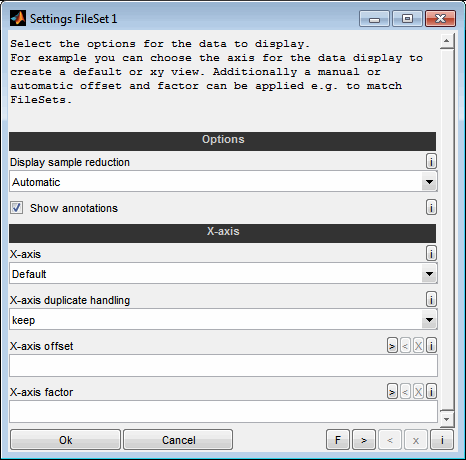
Display sample reduction

To accelerate the display a sample reduction method can be chosen. "Unreduced" means no reduction. Every sample of the loaded data will be displayed. This may slow down the software immensely. "Automatic" lets the program choose a suitable reduction automatically, which is then dynamically adjusted to the actual view avoiding aliasing effects. So even in automatic mode you will be able to see spikes and the data value range.

To switch between "Automatic" and "Unreduced" use the corresponding menu item.

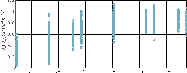
You only need to choose the "Unreduced" option if you need to look at values between the minimum and maximum value for one axis point. This is especially important if you turn on the line markers and turn off the lines itself (e.g. when using xy view). With display option "Automatic" you will only see a reduces set of data values.

The following two figures show the difference in visualization using "Unreduced" (1. figure) and "Automatic" (2. figure) when creating a xy view with markers only.

Show annotations

Select whether to display annotations derived from the files to load like e.g. user pause comments or trigger events. Depending on the data loading mode you will be asked for detailed options afterwards or the options will be adopted from an existing FileSet. See “Add annotations from file” for details.
X-axis

Choose the channel to use as x-axis to get a x/y diagram. "Default" is the standard axis from data load procedure which is mostly the time.

To create a x/y view select one of the loaded channels to be the x-axis. If the chosen channel (for x-axis) is not monotonously increasing, the values will be sorted automatically. Therefore, it is often useful to turn on the line markers, turn off the lines itself and to switch the display option to "Unreduced". See the previous section to understand the effect of this setting.
X-axis duplicate handling

In case the x-axis contains duplicate values you can select how to handle them.

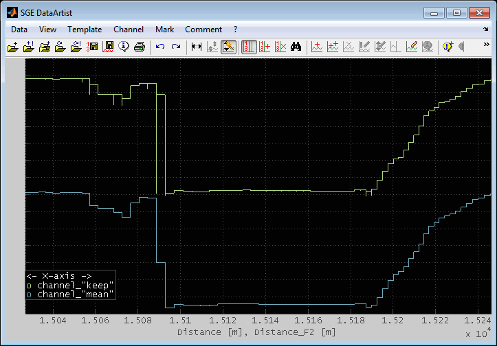
keep: Maintain all duplicate values. The display will show all or only only the maximum and minimum value depending on the “Display sample reduction” setting and there channels a line display will have vertical steps.

mean, max, min, mean: Calculate a statistical value of duplicate axes values. The sample count will reduce accordingly.

See the following figure for a comparison of the “keep” and the “mean” setting for the same data channel.

X-axis offset / factor

Define a offset and factor for the axis values of the loaded data. This can be used to synchronize the FileSets. You can enter an numeric value or "auto" to start a wizard for an automated matching of two channels to find the optimum offset. "keep" means to adopt the values of the available data. This is only valid if you replace a FileSet or load from template.

The offset can also be adjusted later on in the graphical view by dragging the channels. The factor must be > 0.

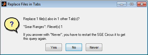
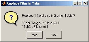
You can also replace a FileSet (Ctrl + o). Just mark one channel of the FileSet and choose “Replace FileSet”. The channels and load data options are asked and prefilled with the information from the FileSet to replace. When replacing a FileSet while multiple Tabs exist sharing the same files you will be asked whether to replace the files for all Tabs.

To speed up data loading use the Add/Replace FileSet quick feature (Alt + o, Alt + Shift + o). Only the file(s) to load will be asked then. The options will be maintained. Therefore it is easy to replace or add files while keeping all display settings, calculated channels etc. In case a channel is selected its FileSet will dictate the options to use. In case no channel is selected (Esc) the first FileSet will be used when adding a new FileSet. To replace a FileSet a channel must be selected when multiple FileSets exist.

4.2 Delete FileSet

To delete all channels of the FileSet and therefore the entire FileSet use the corresponding menu item or keyboard shortcut (Ctrl + Del).

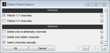
FileSets

Select the FileSet(s) to delete all channels for from the current view. Deleted channels will also be removed from overview and GPS view. Remember that the options below must also apply for the channels to delete.
Delete only invalid/empty channels

If this option is activated, only channels that contain completely invalid values (NaN, inf) or are empty are deleted.

Only channels of the FileSets selected above are taken into account.
Delete only hidden channels

If this option is activated, only hidden channels are deleted.

Only channels of the FileSets selected above are taken into account.
Select channels manually

If this option is activated, you then have the option of manually selecting the channels to be deleted again in a dialog that is preset according to the criteria specified here.

Only channels of the FileSets selected above are taken into account.

4.3 Drag and drop, paste clipboard

In addition to using the file load dialog, you can load sessions, templates and data files by using drag and drop or the clipboard. To do this, one or more files can be dragged directly to a DataArtist session or inserted via keyboard shortcut (Ctrl + v). It is also possible to copy files directly to the clipboard as well as strings containing the file names line by line.

Adding data files this way will create one or more new FileSets. Choose how to handle the file(s) to add. You can create a new FileSet or replace an existing one.

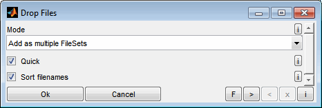
Add FileSet

The files will be added as a single new FileSet by concatenating the files sequentially.
Add as multiple FileSets

The files will be added as a multiple new FileSets. One file gives one FileSet. The channels and options will be asked only once. If “Quick” is selected they will be adopted from an existing FileSet.
Replace selected FileSet

The files will be added as a single new FileSet and they replace the FileSet of the selected channel.
Replace all FileSets

The files will be added as a single new FileSet and they replace all existing FileSets.
Quick

When selecting “Quick” no options will be asked from the second FileSet. They will be adopted from the existing FileSet. They will be adopted from an existing FileSet.
Sort filenames

Depending on the operating system, the order of the selected files differs depending on how they were sorted and selected in the file selection dialog. With this option it is possible to specify the order sorted by file name independently of the selection.

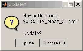
4.4 File update

If you already have loaded a FileSet and use the Replace functionality it is automatically checked for an update. This means that if in the directory of the currently loaded file exactly one file with the same ending exists that has a newer file date this one is proposed to be loaded directly without asking options.

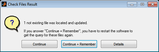
4.5 Check files

The files the data was loaded from is remembered and will be used e.g. to prefill the dialogs when reloading data. They can also be displayed using the data info (Ctrl + Shift + i).

It may happen that files have been renamed or moved during the work or after reloading a session. Use the “Check files” option in this case to search the missing files and update their names and path automatically. Remember that sometimes it is not possible to find missing files. Especially all files must be located in the same directory. The option “Continue + Remember” allows you to save search results and apply them quickly next time without prompting. To reset these saved replacements, the software must be restarted or the corresponding option must be used when the message after automatic replacement is displayed.

4.6 Delete data

Data may also be deleted (Ctrl + d). This is mainly useful to reduce the size of session files to save or to avoid Out Of Memory errors when handling big amounts of data. Beneath deleting single channels (Del) or FileSets (Ctrl + Del) it is also possible to delete data e.g. inside/outside the actual view or inside/outside the marks.

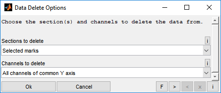
Sections to delete

Choose the sections to delete the data from.
- Screen view
- Outside screen view
- All marks (if any)
- Selected marks (if any)
- Unmarked sections (if any marks)
Channels to delete
- Selected channel
- All channels
- All channels of FileSet
- All channels of common Y axis
- Select channels manually

Channels without remaining data will be deleted afterwards. Deleting data cannot be undone. Deleting data is not remembered in a template file. So loading a template from a session with data deleted will again load the complete data.

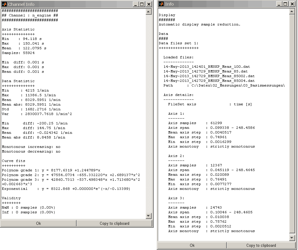
4.7 (Data) Info

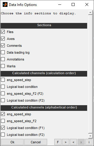
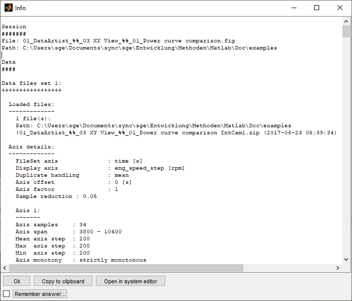
You can display some information about the loaded data (Ctrl + Shift + i) like file names, comments, axes details, data loading history and calculated channels. This may be helpful to document the work done. In case of multiple loaded files you can also see the axis order of the files from this information.

Calculated channels will be shown by opening them in the CalcGuide. This is just for display purpose. Modifications done in the CalcGuide will be discarded. In order to be able to find calculated channels quickly but also to be able to view the sequence of the calculation, they are displayed unsorted and sorted.

The data can be copied to the clipboard.

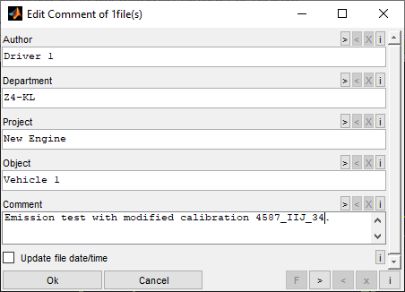
4.8 View / edit comment

For some file formats (MDF, Keihin, 2D) editing of the file comments is supported (Ctrl + m). In case of multiple loaded files you will be asked which file to edit. You can also choose all and the comment of all files will be overwritten with the input.

An option allows you to decide whether the file date is to be updated or left unchanged.

5 Channels

5.1 Add / Delete

You can add channels to a single FileSet (Ins) or to all FileSets at once (Ctrl + Shift + Ins). The added channels will be loaded with the same settings (e.g. logical load condition) as the data already displayed. In case channels should be added to all FileSets the selected channel dictates the FileSet whose channels are presented for channel selection.

The FileSet to add the channels is displayed in the heading of the channel selection dialog.

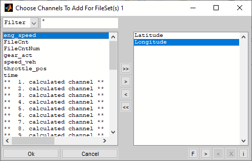
When channels are added that are already loaded but are hidden they will be made visible.

It is also possible to delete single channels (Del) or all (Ctrl + Del) channels of the FileSet that correlates to the selected channel from the display. Deleted channels will also be removed from overview and GPS view. Deleting a FileSet (Ctrl + Del) offers additional options, e.g. to delete only empty, invalid or invisible channels. Since it also provides an option to select channels, it can also be used to delete only parts of a FileSet.

5.2 Select / Search channel

Exactly one channel can be selected at a time. The selected channel is underscored in the cursor and highlighted through a increased line width of its data curve.

To select a channel you can click to its data curve or its name in the cursor. You can also perform a long click to highlight and display the channel exclusively for a short time.

It is also possible to select a channel by uninterrupted typing of its name in lowercase letters. After stopping to type a matching channel will be searched and the first match will be selected and display exclusively for a short time. Use * as a wildcard character.

The state of exclusive channel display can be extended using the Shift key. After releasing the Shift key the previous state is restored.

Alternatively a channel may be selected using the corresponding menu item (F3).

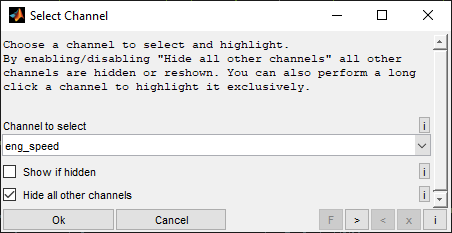
Channel to select

Choose the channel to select and highlight. The channel will shortly be shown exclusively by hiding all other channels and will be underscored in the cursor list.
Show if hidden

The selected channel will be made visible if it is hidden currently.
Hide all other channels

If enabled all channels except for the selected one will be hidden. If disabled the channels that were hidden the last run will be reshown.

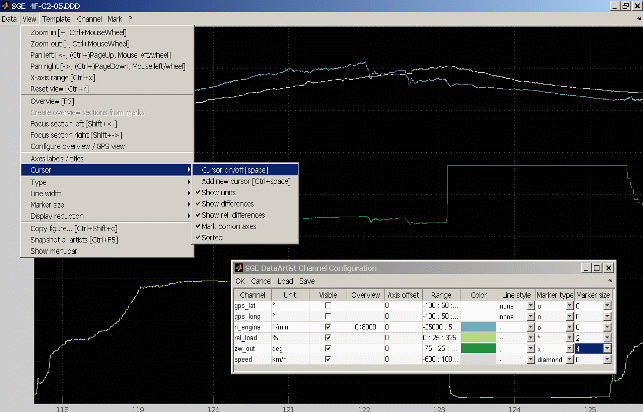
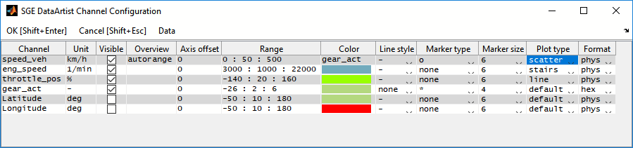
5.3 Channel configuration

Various display options can be modified using the channel configuration dialog (F4). The input can be saved to and loaded from a file using the “Data” menu to allow quick access to commonly used settings. Also quick access to the latest configuration is available in the “Data” menu and an options to save the current configuration as a default for channels loaded at a later time. This way default configuration can be generated e.g. from an old session.

Range

For automatic spacing enter the limits as numerical values separated by spaces. For limits and spacing enter a valid vector syntax with colons. Maximum and minimum must not be equal.

Examples:

0 100 (From 0 to 100 with automatic spacing)
0 : 10 : 100 (From 0 to 100 with spaces of 10)

If you modify the range of a channel joining a common Y axis you will be asked whether to modify also all other channels of the common Y axis or to remove the channel from the common Y axis.

Overview

Specify the minimum and maximum limits separated by colon or space. For full range enter "a" or "auto". Maximum and minimum must not be equal.

Examples:

0 100 (From 0 to 100)
0 : 100 (From 0 to 100)

Plot type

The plot type can be adjusted to display channels as stairs, line or stems. Also a default setting is available. This can be modified using the menu item “Default plot type”.

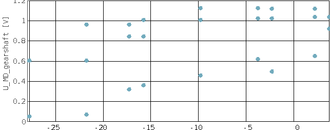
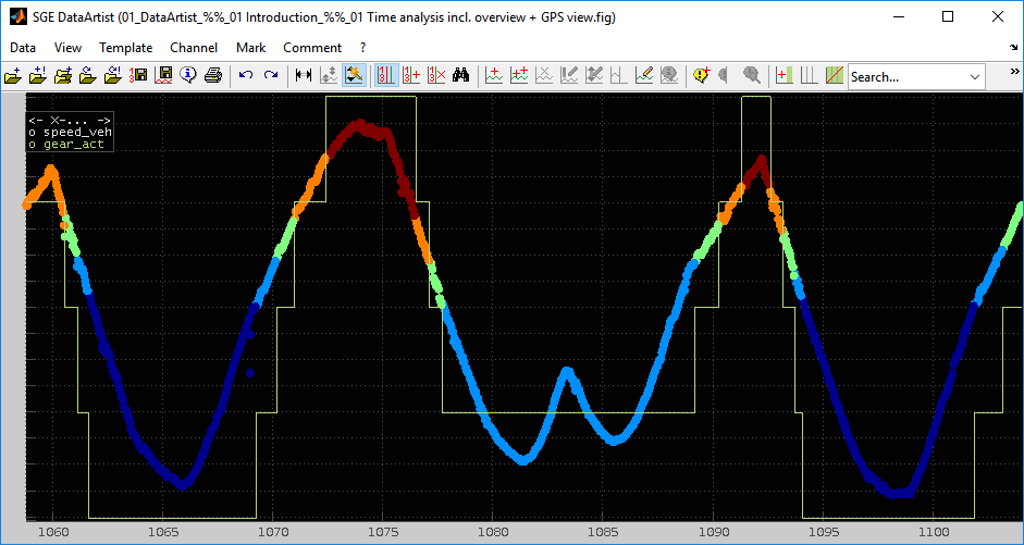
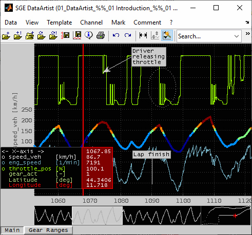
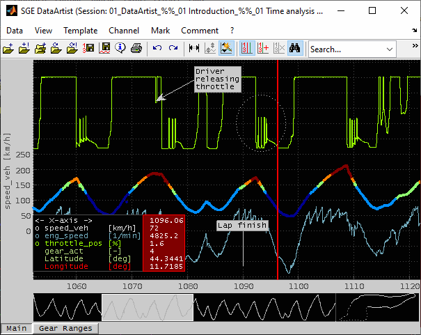
The “scatter” setting is used to display data points colored accordingly to the values of a color source channel. In this case you do not select a color for this channel but the color source channel instead. Depending ob the scale (y-axis range) of the color source channel the colors a chosen for the scatter channel automatically. A scatter must have a marker type o, square, diamond, ^, v, <, >, pentagram or hexagram. As an example in the following figure the speed_veh channel is colored by the gear_act channel.

Format

The format does affect the display of the data values inside the cursor tables. Choose between physical, hexadecimal, binary and octal format.

Be aware that for all formats except for physical the data values are rounded towards the nearest integer and limited downwards to zero.

5.4 Color

Channel color

You can modify the color of each channel by a color selection dialog (Shift + enter) or quickly by switching to next / previous color (Shift + n, Ctrl + n). In case the channel is a scatter channel you will be asked for the color source channel instead of the color itself.

The colors are remembered as a preference for the channels names. So if channels are loaded at a later date the colors will be reused if the channels names are already registered.

Color FileSets

The option “Color all FileSets” will automatically color channels of multiple FileSets accordingly to the color of the corresponding channels of a master FileSet. To find corresponding channels the names must only differ after an underscore (gear → gear_F2, gear_Var1 → gear_Var2). The colors will get lighter with higher FileSet numbers. This way you can easily come to a clearly visible file comparison by coloring the first FileSet with strong colors and the choosing this option.

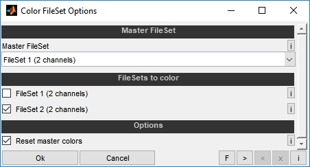
Master color FileSet

Select the FileSet to use as master for the colors to apply. Its colors will remain unchanged unless you use the "Reset master colors" option.
FileSets to colorize

Select which FileSets to apply the colors to that will be derived from the master FileSet selected above.
Reset master colors

Select whether to reset the decolorized colors of the master FileSet before applying colors to the other FileSets.

5.5 Range

A set of features is available to adjust the channels Y-ranges. The ranges are remembered as a preference for the channels names. So if channels are loaded at a later date the ranges will be reused if the channels names are already registered. If these ranges would lead to place the data loaded completely outside the screen range they will get discarded.

Range / common Y axes settings

The range and tick dimension of the y-axis can be set for each channel separately. Additionally multiple channels can be assigned to a common y-axis using the channel range dialog (Enter, Mouse double click to channel or cursor entry).

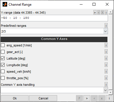
Y-range

You can provide the limits only or the limits and the spacing. For the limits only enter them as numerical values separated by spaces. For limits and spacing enter a valid MATLAB vector syntax with colons. If the limits difference does not match a multiple of the spacing the max. limit is modified accordingly. The maximum limit can be lower than the minimum to create a reverse axis. Maximum and minimum limit must not be equal.

These Y-range and scaling can also be accessed by keyboard shortcuts or mouse gestures (Ctrl + +/-, Ctrl + Up / Down).

Examples:

0 100 (From 0 to 100 with automatic spacing)
0 : 10 : 100 (From 0 to 100 with spaces of 10)
100 : -10 : 0 (Reverse axis from 100 to 10 with spaces of 10)

Predefined ranges

You can alternatively choose from a list of predefined ranges. For example 2/5 means that the y-axis is split in 5 parts and the channel is placed in the 2nd one from the bottom. If "Smart range" in the menu is turned on the limits will be adjusted to some round values. These actions can also be accessed by keyboard shortcuts (Ctrl + 0..9, Ctrl + Shift + 0,ß). The selection in the predefined ranges field will only be considered if values for limits and spacing are not modified.

Common Y axes

With the check boxes you can choose the channels that should use one common y-axis. Initially all channels sharing the axis of the selected channel are checked. When you check additional boxes these channels will be scaled to the axes of the already checked channels. If you uncheck boxes these channels are set to a separate (new) axis. If you uncheck multiple channels all of them will be set to one new common Y axis.

A common action for all channels can be performed to group all channels to one single common Y axis or to remove all common Y axes correlation and use separate axes for the single channels. When this option is used the checkboxes above will be ignored.

Additionally a channel can be added quickly to the common Y axis of the currently selected channel (Ctrl + Mouse click).

Range adjustment using mouse

The positioning and range setting can be done very easily using the mouse.

Move channel in y-direction

By dragging a selected channel with the right mouse button you can move it in y-direction.
Zoom channel in y-direction

By zooming a selected channel with the left mouse button you can adjust its y-range. The following figure illustrates the zooming behavior. In order to avoid misunderstandings, the zoom is only performed when parts of the data of the channel are later within the screen. If the entire channel were outside, it will not be scaled. When scaling using the mouse, all channels of a common Y axis are scaled.
Scale channel in y-direction

By dragging with the right mouse button while Ctrl button is pressed you can scale the selected channel it in y-direction. If you click exactly to the channel before dragging this channel value will remain its position on the screen while the parts above and below will be scaled. Otherwise the mean value of the channel will remain its position.

All operations refers to the selected channel. All channels of a common Y axis will be handled commonly.

Smart range setting

In the channel menu you can check a “Smart range” option. In this case the y-axis range is rounded to even values when using the predefined ranges or mouse actions.

Range adjustment using keyboard shortcuts

Several keyboard shortcuts are supported to quickly adjust the channels Y-ranges (Ctrl + 0..9, Ctrl + Shift + 0,ß, Ctrl + +/-, Ctrl + Up / Down). See “Keyboard shortcuts, mouse gestures“ for a full list of supported shortcuts.

5.6 Show / hide

Channel can be hided in the graphical view (Ctrl + h). Depending on the configuration of the cursor they are anyway listed in the cursor table to allow data evaluation.

It is also possible to hide/show all channels sharing a FileSet at once (Ctrl + Shift + h) or all channels sharing a common Y axis (Shift + h).

Additionally a hidden channel can be shown quickly by using Ctrl + Mouse click. Remember that this also adds the channel to the common Y axis of the currently selected channel.

5.7 Shift

You can shift one or all channels of a FileSet (Ctrl + shift + x, Mouse right button drag). This means that its axis values are modified with an offset. The mode can be absolute or relative. When relative is chosen the input value is added to the actual offset. When absolute is chosen, the actual value is ignored and the total offset is set to the input value. Shifting channels may also be done using the Channel Configuration dialog (F4).

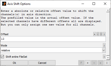
This feature is e.g. helpful is you want to correct emission analyzer time offsets to synchronize emission channels to ECU measurement channels.

5.8 Style channels automatically

This feature (Shift + F4) will automatically style channels depending on search patterns related to the channel names. You can use rules to select channels relating to their names and apply colors, markers, line style, ranges and common Y axes settings.

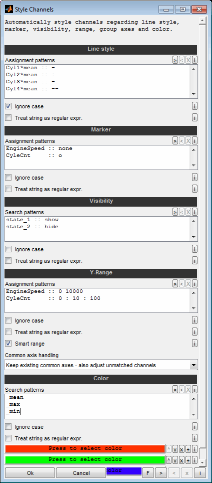
Line style

You can use rules to automatically set line styles for channels in relation to their names. One rule is given per line. The string to look for and the line style are separated by two colons, like "EngineSpeed :: ;". The assignment is done in the order of lines from top to bottom. Use * as a wildcard.

Valid line styles are:

- solid line

-- dashed line

-. dash-dot line

: dotted line

none no line, only allowed with marker active

Example:

Cyl1*mean :: -

Cyl2*mean :: --

Cyl3*mean :: ;

Cyl4*mean :: :

CylCnt :: none
Marker

You can use rules to automatically set markers for channels in relation to their names. One rule is given per line. The string to look for and the marker symbol are separated by two colons, like "EngineSpeed :: o". The assignment is done in the order of lines from top to bottom. Use * as a wildcard.

Valid marker symbols are:

none no marker

+ plus sign

o circle

* asterisk

. point

x cross

^ upwards triangle

v downwards triangle

< left triangle

> right triangle

s square

d diamond

p pentagram

h hexagram

Example:

EngineSpeed :: o

Throttle :: *

CylCnt :: none
Visibility

You can use rules to automatically show/hide channels in relation to their names. One rule is given per line. The string to look for and the visibility status are separated by two colons, like "EngineSpeed :: hide". The search is done in the order of lines from top to bottom. Use * as a wildcard.

Valid visibility status are:

show Show matching channel

hide Hide matching channels

1 Show matching channel

0 Hide matching channels

Example:

EngineSpeed :: show

Throttle :: hide

Cyl1*Mean :: hide
Range, common Y axes

You can use rules to automatically set the Y-range for channels in relation to their names. One rule is given per line. The string to look for and the range definition are separated by two colons. You can provide the limits only or the limits and the spacing. Additionally you can provide a relative range part to fill by the matching channels.

For limits only enter them as numerical values separated by spaces.

Example:

Cyl1*mean :: 0 100 (From 0 to 100 with automatic spacing)

For limits and spacing enter a valid vector syntax with colons. If the limits difference does not match a multiple of the spacing the max. limit is modified accordingly. The maximum limit can be lower than the minimum to create a reverse axis. Maximum and minimum must not be equal.

Example:

Cyl1*mean :: 0 : 10 : 100 (From 0 to 100 with spaces of 10)

Cyl2*mean :: 100 : -10 : 0 (Reverse axis from 100 to 10 with spaces of 10)

For a relative range part enter the part and range separated by a /.

Example:

Cyl1*mean :: 1/4 (First quarter from the bottom)

Cyl2*mean :: 2/4 (Second quarter from the bottom)

Cyl3*mean :: 2-3/4 (Second to third quarter from the bottom)

Cyl4*mean :: 1/1 (Fill entire screen)

Cyl5*mean :: 1 (Fill entire screen)

When assigning the ranges you can decide whether to adjust the limits entered to some round values (smart range) or to exactly set the entered values.

Channels sharing the same ranges can join a common Y axis. By modifying the ranges common Y axes may be concerned. Different modes are available to handle the common Y axes when applying ranges automatically.

Adjust common Y axes if any

When a channel range is modified by automatic assignment and the channel joins a common Y axis with other channels, all other channels ranges will also be adjusted to maintain the common Y axis.
Add to existing common Y axes

When a channel range is modified by automatic assignment all existing common Y axes will be checked for a matching range. If a match is found the channel will be added to the common Y axis.
Create new common Y axes

For the channels modified common Y axes will be created if some of them have the same range after automatic assignment. The existing common Y axes will not be modified.
Do not create common Y axes - keep existing common Y axes

For the channels modified no common Y axes will be created. All of these channels will have an independent axis even for channels with the same range. The existing common Y axes will not be modified.
Do not create common Y axes - discard all existing common Y axes

For the channels modified no common Y axes will be created. All of these channels will have an independent axis even for channels with the same range. Additionally all existing common Y axes will be removed and the correlating channels will get independent axes.

Color
You can use rules to select channels relating to their names and apply a common color. One rule/color per line. The number of lines must agree with the number of color selection buttons below. Color buttons can be added, removed and reordered using the small buttons on the right. The assignment is done in the order of lines from top to bottom. Use * as a wildcard.

Example:

EngineSpeed

Cyl1*mean

For all assignments you can decide whether the string interpretation should be case sensitive and treated as a regular expression.

5.9 Channel info

If a channel is selected you can get information regarding its source, values and axis by the channel info (Ctrl + i). Some statistical values of the currently visible axis section of the channel, min, max, mean, std values and curve fits are displayed. This allows quick determination of e.g. the underlying data files, FileSet number, data gradients, mean values and standard deviations. The information is calculated from the channel data within the current x-axis range. Adjust the visible area accordingly before requesting this info to ensure to get the information desired. The display of this dialog may last long in case of channels with big data amounts.

Since the calculation can be time-consuming, there is the possibility to close the waiting bar. The data calculated until then will be displayed.

5.10 Rename

Channels are handled with the names loaded from the data files. For FileSets > 1 automatically extensions (_F2) are added.

You can rename the channels. Either individually when a channel is selected (F2) or using replacement patterns (Ctrl + F2).

The names must be unique within the loaded channels. If you need the name to agree with the ASAP MCD rules it must consist of a-zA-Z0-9[]_. only with a max. length of 32 characters.

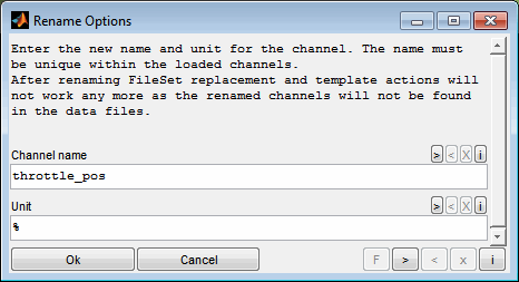
When renaming the selected channel a dialog allows to modify the channel name and its unit.

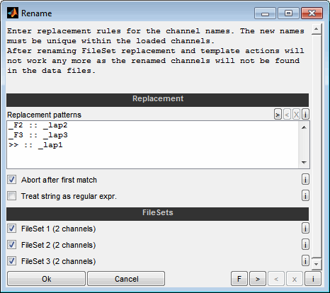
Replacement patterns

When renaming the channels using replacement patterns they must be given one rule per line. The string to look for and the replacement are separated by two colons, like "EngineSpeed :: RPM". A special meaning have "<<" and ">>". In this case the replacement pattern is appended to the beginning (<<) or end (>>) of all channels of the selected FileSets. This is used to append without replacing. E.g. for FileSet1 channels - when no _F2 is available to replace.

Examples:

EngineSpeed :: RPM
_F2 :: _recording2
>> :: _recording1 (append to the end)
<< :: recording1_ (append to the beginning)

The replacement is case sensitive and done in the order of lines from top to bottom.

Abort after first match

If enabled the replacement for a channel will be aborted after the first rule leading to a change. Otherwise all replacement rules will be applied sequentially.
Treat as regular expression

If the corresponding check box is set the strings are interpreted as regular expression.

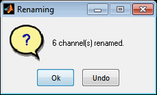
After the editing was done a message will inform about the channel name modification and allows to undo the changes.

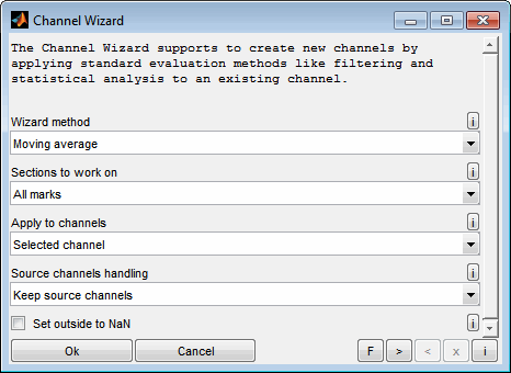
5.11 Channel wizard

The channel wizard allows to create new channels by performing common tasks (like filtering, statistical evaluation, curve fitting) to the loaded channels.

Wizard method
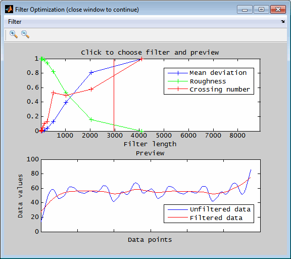
- Moving average filter
  
  A moving average can be applied using a graphical preview GUI. Choose the filter length in the upper diagram to see the result in the lower diagram. You can use the zoom buttons to adjust the view of the lower diagram and keyboard shortcuts to adjust the filter length.
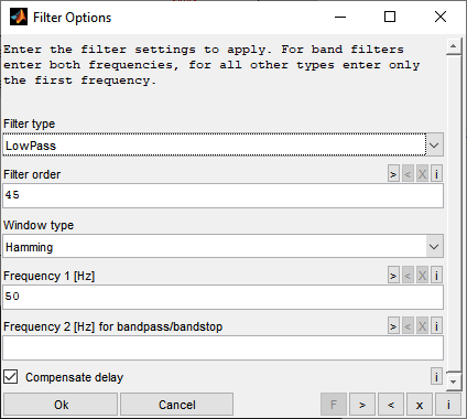
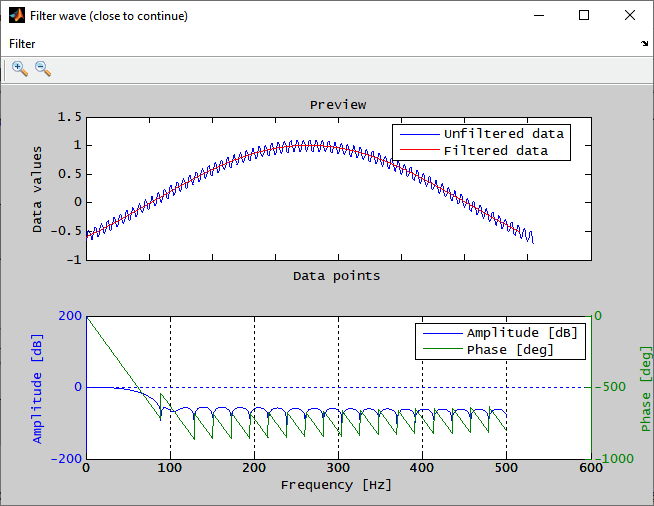
- filter (digital FIR)
  
  A digital FIR filter can be applied using a graphical preview GUI. Choose the filter settings to see the time and amplitude/phase response in the diagram.
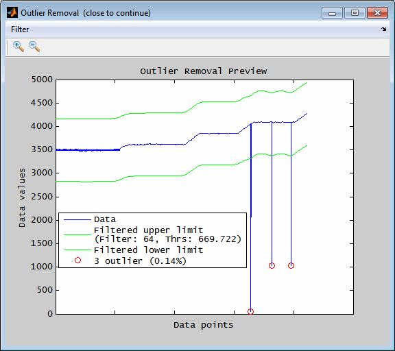
- Remove outliers
  
  Outliers are searched for that lie outside a definable band around a filtered course of the data. In addition, outliers are detected by absolute thresholds. The data, the band around the filtered course and the detected outliers are displayed and can be conveniently adjusted by keyboard shortcuts until the result is satisfactory. Then the window must be closed and the outliers are replaced by invalid values (NaN) or interpolated between valid neighbors if any.
- Mean / max / min value
  
  The resulting channel data values will be the mean / max / min value of the source channel.
- Cumulative sum (relative)
  
  A cumulative sum of the channel starting at zero is calculated. When relative is chosen the sum is scaled to the max. value and therefore ends at one.
- Mean / max / min of duplicate axes values
  
  This method is used to handle multiple values at a single x-axis point. So if the channel contains multiple values at one axis point, you can calculate the mean / max / min value of all data values with the same axis value. This especially useful in x/y view mode to calculate e.g. mean indicating cycles.
- Polyfit / Exponential fit
  
  Curve fits of the channels to work on can be done. The coefficients and determination criteria values are printed to the console.
- Linear detrend
  
  A linear curve is fitted to the data and then subtracted from the data. This can be used to compensate drifting data.
Sections to work on

You can decide to which part(s) of the data you want to apply the method. This can be the whole file or sections of it defined by marks or the screen view.
Apply to channels

You can decide to apply the filter/method to the selected channels, all channels or the channels of the current FileSet/common Y axis. Alternatively you can select the channels to apply to manually.
Source channel handling

You can decide to delete, hide or replace the source channels after creating the new channels. Delete and replace are similar with the difference that for "delete" the new channel will have a new name indicating the modification while for "replace" the name of the new channel will be the same as the source channel.
Set outside to NaN

You can set the parts of the data that does not apply to the sections to NaN what makes them invisible.

Channels created by the wizard will not give reliable results when loading a template – especially when using logical load conditions. It is recommended to add the channels directly as calculated channels when loading the data if templates should be saved.

5.12 Analyze

The “Analyze” menu supplies some commonly used tasks to analyze the data of the selected channel.

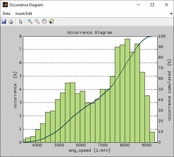
5.12.1 Histogram

A 2D or 3D histogram view of one or two channels will be displayed. The histogram data can be exported to different graphics and data formats. The following options are available:

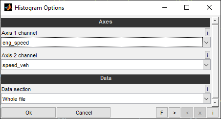
Axes channels

Choose the channels to use for the axes of the histogram. When selecting only one channel a 2D histogram will be created. From two selected channels a 3D histogram will be created. When the second channels axis does not match the axis of "Axis 1 channel" it will be interpolated automatically. The interpolation method depends on the plot type of the channel. "line" type will use linear interpolation while all other plot types look for the next value to the left axis side. The plot type can be set in the "Channel configuration".
Data

Choose the sections to consider depending on the following axis options:

Whole file
Screen view
All marks (if any)
Selected marks (if any)
Unmarked sections (if any marks)

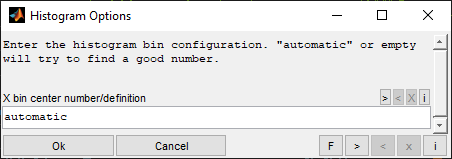
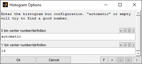
X bin center definition

Enter an expression to define the histogram bin position. This can be the number of bins as a single numeric value, a vector of bin position values or "auto" for automatic detection of a suitable bin number. In case a vector is given the bin borders are in the middle of the bin positions. Therefor the bin positions are not necessarily the center positions in case of unequal spacing.
- Examples:
  
  10 10 bin with equally spaced distance.
  
  auto Automatic detection of a suitable bin number.
  
  [1 2 5 10 20] 5 bin with given positions.

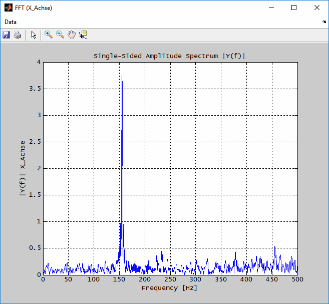
5.12.2 FFT

One or more FFT analysis of the actual selected channel data will be created. For the FFT to have a meaningful frequency axis the data of the channel to analyze must be sampled with constant frequency and the axis unit must be seconds. If this is not the case, the FFT will be calculated for an average sampling rate and you will be notified accordingly. If the source data deviates from this sampling rate or the axis unit is not seconds, you must interpret the frequency axis yourself.

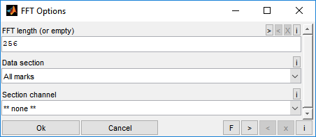
FFT length

Enter the number of FFT axis samples to create. The value must be in the range 2..2^12 and will be rounded to the next power of 2 automatically. Leave empty to determine automatically. The resulting display will only include the positive frequency part - so the resulting axis samples are n/2+1.

Data section

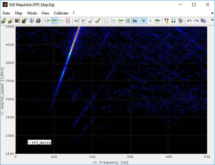
Select the sections to create individual FFTs for. In case multiple FFTs are to be created these will be displayed as a map with one axis resulting from the frequency and the other from the section channel.

As an example you could split an engine speed ramp with noise recording into marks covering separate engine speed ranges and than create separate FFts of the noise for the single marks.

The following sections are available:

Whole file
Screen view
All marks (if any)
Selected marks (if any)
Unmarked sections (if any marks)

Section channel

When selecting multiple sections to create FFTs for you can assign a section channel. For each section the mean value of this channel will be used as axis value for the resulting FFT map.

In our example of the engine speed ramp with noise recording select the engine speed as section channel to display its values with the map.

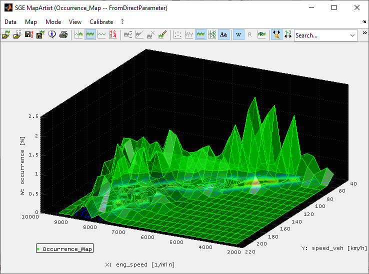
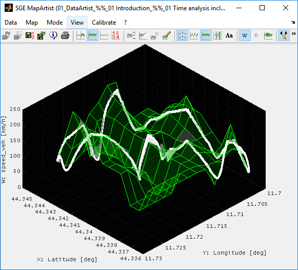
5.12.3 MapArtist

Three channels of the loaded data can be send to the SGE MapArtist to create and visualize a map. The following options are available:

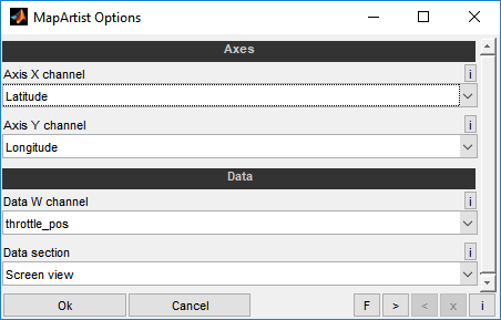
Axis X/Y channel

Choose the channel to use for the X axis of the MapArtist. If this channels axis does not match the one of the axis W channel it will be interpolated automatically. The interpolation method depends on the plot type of the channel. "line" type will use linear interpolation while all other plot types look for the next value to the left axis side. The plot type can be set in the "Channel configuration".
Data W channel

Choose the channel to use for the W data of the MapArtist.
Data section

Select the sections to collect the data from.
- Whole file
- Screen view
- All marks (if any)
- Selected marks (if any)
  
  Unmarked sections (if any marks)

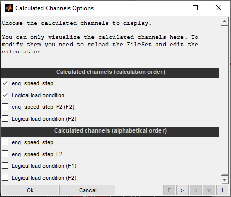
5.13 Show calculated channels

The loaded calculated channels can be displayed. You can only visualize the calculated channels here. To modify them you need to reload the FileSet and edit the calculation. In order to be able to find calculated channels quickly but also to be able to view the sequence of the calculation, they are displayed unsorted and sorted.

5.14 Split channels

Split channels to create individual channels for single sections of the data loaded. This makes it possible, for example, to conveniently superimpose individual sectors of the data loaded without loading multiple FileSets. Common use cases are the superposition of the single laps of a race track recording or the superposition of single combustions of a cylinder pressure indication recording.

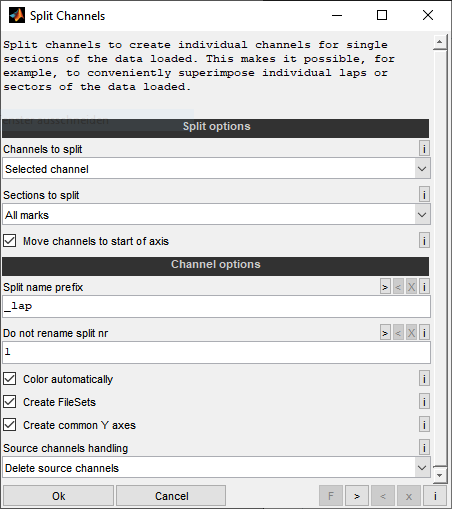
Channels to split

You can decide to split the selected channel, all channels of the selected FileSet or all channels of the common Y axis of the selected channel. Alternatively you can select the channels to apply to manually.

Due to the very powerful possibilities for mark detection, the channel split can be carried out efficiently using very different possibilities, like logical marks or ramp detection.
Sections to split

You can decide to split the data at the mark bounds, cursor positions or the actual x-axes borders.
Channel name prefix

Enter a string to indicate the single split sections. The section number will be added automatically. E.g. "_sect" leads to "ChannelName_sect1/2/3"
Do not rename split nr

One split can be selected whose channels are not renamed. This makes it possible to maintain e.g. the overview and GPS view that are related to specific channel names. Enter a single number of the split to keep its channels names, e.g. 2 for the second split section.
Move channels to start of axis

You can decide to shift the new channels to start at the minimum value of the x-axis data. In this way it is possible to create a superposition of the channels.
Color automatically

You can decide to automatically color the split channels accordingly to the color of the corresponding first channel. The colors will get lighter with higher split numbers. This way you can easily come to a clearly visible comparison of the single split sections.
Create FileSets

You can decide to automatically create separate FileSets for all split channels of one section. This makes it easy to handle the channels of a split, for example, when switching visibility or deleting a split.
Create common Y axes

You can decide to automatically create common Y axes for all split channels of one source channel.
Source channel handling

You can decide to delete or hide the source channels after splitting. This can affect only the channels that serve for the split or all channels existing before the split.

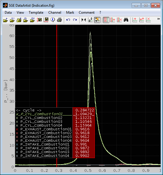
The following example figures show the superposition of the single combustion cycles of a pressure indication recording. The split was done based on the marks set to cover the single combustions.

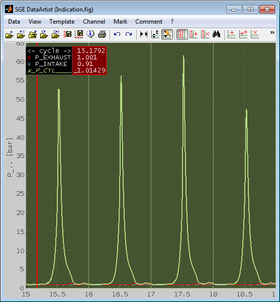
5.15 Reduce data

This function allows data reduction by removing data points so that a given tolerance is not exceeded. As many data points as possible will be removed without the reduced channel deviating more than this tolerance from the original one.

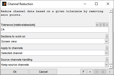
Tolerance [relative/absolute]

Select the tolerance for reducing the data. As many data points as possible will be removed without the reduced channel deviating more than this tolerance from the original one. For this comparison, all data points of the original channel are considered. The tolerance can be given as an absolute value in the unit of the channel or as a relative percentage.

Example:

0.1 -> Reduce without exceeding 0.1 deviation

1% -> Reduce without exceeding 1% deviation
Sections to work on

You can decide to which part(s) of the data you want to apply the reduction.
Apply to channels

You can decide to apply the reduction to the selected or all channels. Alternatively you can select the channels to apply to manually. All channels are treated separately for the reduction.
Source channel handling

You can decide to delete, hide or replace the source channels after creating the new channels. Delete and replace are similar with the difference that for "delete" the new channel will have a new name indicating the modification while for "replace" the name of the new channel will be the same as the source channel.

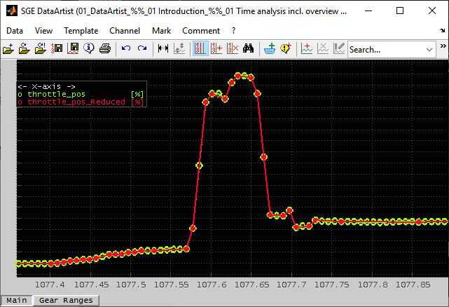
The following example figures show the reduction of a channel with a tolerance of 2%.

5.16 Create mark indication channel

If marks are existing you have the option to create a channel that will have a value of one inside the marks and zero outside. This channel can be used e.g. as a logical load condition according to the marks or to recreate the marks easily in a loaded template.

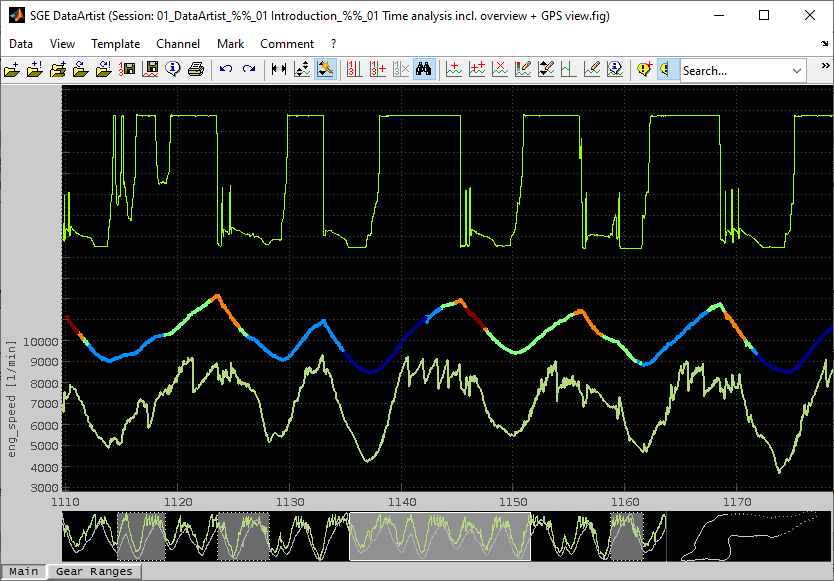
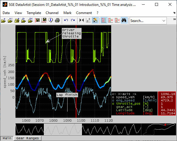
6 View

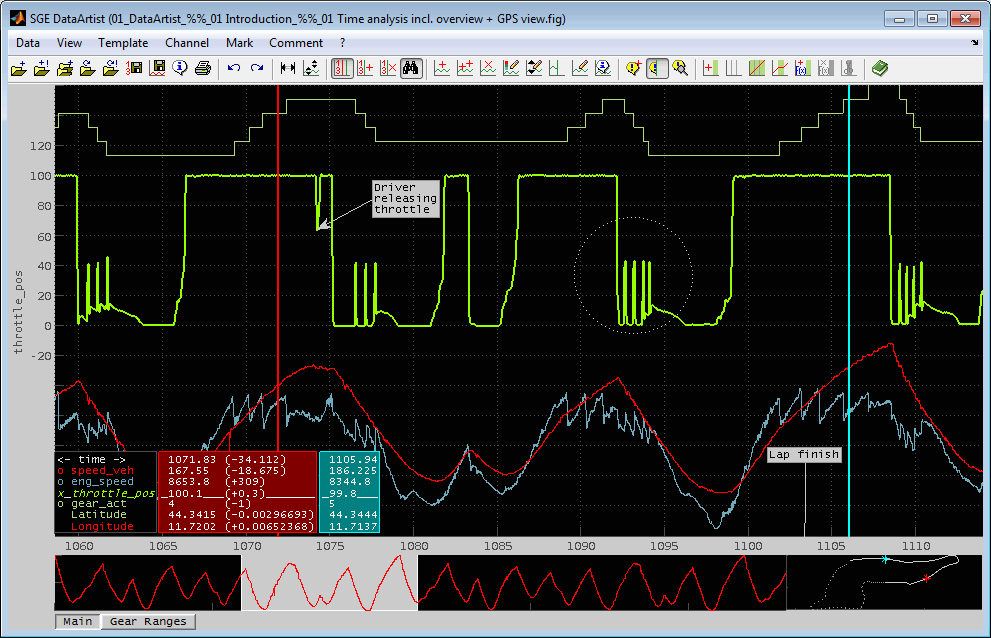
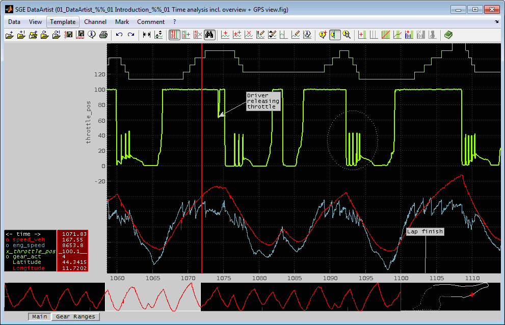
The DataArtist window has three main sections. The main view, the overview at the bottom and the GPS view at the right bottom. Overview and GPS view must be activated to be visible (F6).

Using tabs enables to create multiple views in parallel. See section “Tabs”for details.

6.1 Main view

The main view in the top section can be adjusted quickly by using mouse and keyboard shortcuts – e.g. zoom, unzoom (Mouse left button drag, +/-, Ctrl + Mouse Wheel) and panning (Mouse right button drag, (Ctrl + ) ← →, (Ctrl + ) Pageup/down). The view can also be reset to cover the whole axis range using shortcuts (Ctrl + F12, Ctrl + r).

It is also possible to adjust the view to the cursor positions (Shift+space) if exactly two cursors are present and to resize the main view on the left and right end using the mouse to create space for the cursor if these should not overlay the main view.

The display settings can be modified using the following dialog via the “Display settings” menu item.

Window title

This string is displayed at the top of the window above the menu. Leave empty to use an automatically generated standard string.

You have the possibility to customize the string by automatically inserting dynamic values. The dynamic values are enclosed in %% and start with a ? or !. The ! indicates that the value is displayed in any case. The ? indicates that the value is optional. It is only displayed if no optional values are displayed in front of it.

The following dynamic values are available:

Session : Name of the session file

SessionWithPath : Name of the session file incl. path

Template : Name of the template file

TemplateWithPath : Name of the template file incl. path

DataFirstFile : Name of the first data file

DataFirstFileWithPath: Name of the first data file incl. path

DataFilesetNumber : Number of FileSets

DataInfo : Number of files for each FileSet (e.g. 3+1+4)

Tab : Name of current tab

Examples:

"SGE DataArtist" -> fixed string

"SGE DataArtist (%%!Session%%)" -> string + session file

"%%!Session%% %%?Template%% %%?DataFirstFile %%" -> session file (always) + one of template or data file
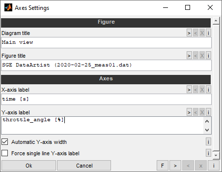
Diagram title

This string will be displayed between the menu and the diagram.
Axes label

The labeling of the x- and y-axis can be modified. However when you select a channel the x- and y-axis will be relabeled and the modified labeling will get discarded. So this input is only useful to create a temporary view.
Automatic Y-axis width

If the width of the Y-axis is determined automatically, the labeling is always completely visible. However, the width of the label and thus of the diagram changes if, for example, another channel is selected. This means that the display must be refreshed. To avoid this, the automatic width can be deactivated. Then the width can be set manually with the mouse dragging the left/right border of the diagram.
Force single line Y-axis label

By default the Y-axis will be automatically labeled with the names and units of all channels assigned to the common Y axis of the marked channel. Therefore the label may consist of multiple lines. This may lead to a repeated width adjustment of the axis and diagram when switching between different channels. To avoid this you may check this option. Then only the marked channel itself will be used for labeling and therefore the label will consist of exactly one line.

Alternatively, the previous option can be used to deactivate automatic width adjustment.

Some display options are available using the corresponding menu items:

Default plot type

You can decide to display the channels by default as stairs, lines or stems. Anyway each channel can be configured individually using the Channel Configuration dialog (F4).
Line width
Font size
Background color
Toggle markers (Shift + z)

Use this menu item to quickly turn on or off markers for the selected channel. If no channel is selected the markers for all channels are toggled.
Toggle markers + lines (Ctrl + Shift + z)

Use this menu item to quickly turn on or off markers+lines for the selected channel. If no channel is selected the markers for all channels are toggled.

6.2 Overview

The overview (F6) always covers the whole horizontal axis range. If the main view shows only a section of it this is displayed in the overview by a white rectangle. The main view and this rectangle are linked. So you can zoom or pan in the main view and the overview rectangle will adjust or you can drag or extend the rectangle using the mouse and the main view will adjust.

Additional rectangles can be created and activated by dragging with the mouse inside the overview. This allows quick switching between main views. Deletion is done by double clicking them.

You can add any number of channels to the overview. By default each channel is scaled to fill the overview. In this case the overview does not allow any data value interpretation or comparison. Using the “Overview / GPS options“ enables you to apply a user defined range also for the overview. It is remembered as a preference and when the channel is used next time in the overview the user defined scale is applied. If you like to re enable the automatic scaling you could enter “auto” or just “a”.

To quickly create a big number or exactly defined overview sections you must first create marks and can then create overview sections from it.

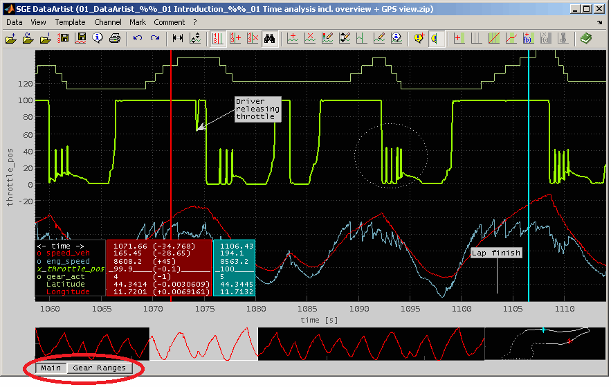
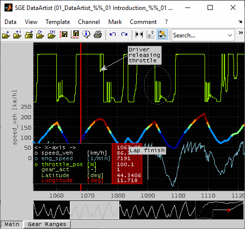
6.3 GPS view

The GPS view is shown when the channels for Latitude and Longitude are set and the overview is enabled. These channels must already be loaded. Even if its called a GPS view it can be used as an all-purpose xy view to display the operating point. If cursors are activated the positions are marked in the GPS view. The actual main view range is indicated by a continuous line.

6.3.1 GPS lap step click

By clicking onto the GPS view the main view is centered to the GPS point clicked. In case the data consists of multiple sections with similar GPS data (e.g. laps on a race track) you can click several times to the same GPS position to jump between the sections (=laps).

6.3.2 Overview / GPS options

Overview and GPS view are configured using the following dialog.

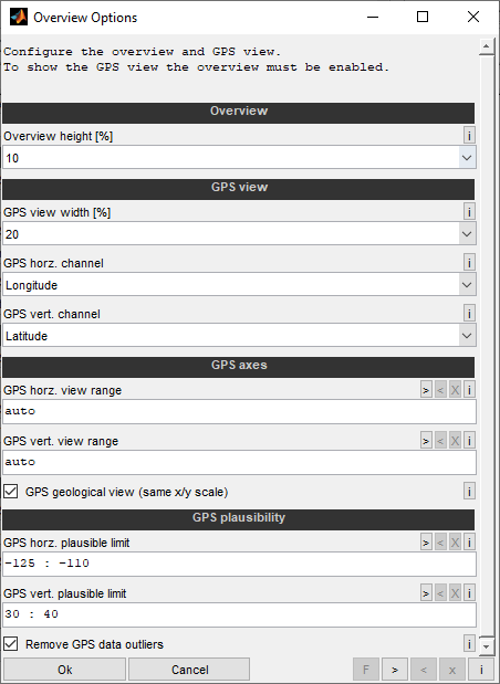
Overview height [%]

Select the vertical part of the window height to cover by the overview-chart.
GPS view width [%]

Select the horizontal part of the window width to cover by the GPS view.
GPS horz./vert. channel

Choose the channel to use as horizontal and vertical values for the GPS view. These channels must be already loaded.
GPS horz./vert. view range

Enter the view range to use for the horizontal GPS axis Choose one of the following proceedings:
- Enter range: Use format "Min : Max". E.g. "35 : 40".
- Leave empty: The range for the channel name will be filled from history if any. If no history entry is found the range will be chosen to match the data range.
- "auto": If you enter the string "auto" the range will be chosen to match the data range.
If the data is messed up by outliers try to use the "Remove GPS data outliers" and "GPS horz. plausible limit" options.
GPS geological view (same x/y scale)

Use the same scaling for both axes for geological representation. If this option is activated, the scaling of both axes is automatically adjusted to each other in such a way that an undistorted geological representation is achieved. The scaling of the x and y axes are then coupled. To freely select the axis limits, this option must be deactivated.
GPS horz./vert plausible limit

Enter a range to detect implausible horizontal GPS data values. Horizontal GPS values outside this range will be discarded. Use format "Min : Max". E.g. "35 : 40".

Use this option if the data is messed up by outliers and the "Remove GPS data outliers" option does not lead to satisfying results. Remember that this option is used to remove implausible values. Use the "GPS horz. view range" option if you just want the modify the GPS view ranges.
Remove GPS data outliers

If enabled outliers will be removed automatically from the GPS data without the need to fill the “GPS horz./vert plausible limit” fields.

6.4 Tabs

Using tabs enables to create multiple views in parallel.

Tabs can be added, copied, deleted, renamed and reordered using the corresponding menu item or the context menu. Use keyboard shortcuts to add (Ctrl + t) and activate tabs (Ctrl/Shift + tab) quickly.

The single tabs are fairly independent. The loaded data, axes ranges, marks, cursors, overview/GPS view configuration does not interfere. Central settings like e.g. font size, background color and cursor settings are shared by all tabs.

By activating the corresponding option the x-axis ranges will be synchronized. This means that the x-axis range is kept when activating another tab. Otherwise each tab maintains its own x-axis range. The option “Sync tab cursors” enables to synchronize the cursor positions of all tabs. If the corresponding option is activated the tab buttons will provide mouseover tooltips containing useful information like the files loaded.

When replacing a FileSet while multiple Tabs exist sharing the same files you will be asked whether to replace the files for all Tabs.

Tabs are also handled by sessions and templates.

6.5 Snapshot

If you work with multiple DataArtist instances in parallel you can quickly import the channels displayed from the other instances using snapshot functionality (F5). These snapshots are static. They cannot be modified and are printed with display resolution. Therefore you will not see all data point when zooming.

All instances of the DataArtist to use for snapshots must be started from the same SGE_Circus.

7 Cursors

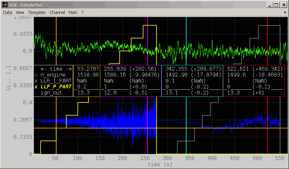
Data cursors allow to analyze data quickly. Just click with the mouse into the axis area besides a channel and the first cursor will appear (Space). You can add any number of cursors (Ctrl + space). The selected cursor is the master. All other cursors display the differences (absolute, relative) from the master cursor besides their own values if activated in the cursor options.

In case of multiple cursors the master can be set by clicking the cursor line, clicking the cursor value table or by using keyboard shortcuts (Shift + 1..9). To center the view to a cursor double click into the cursor value table.

To remove the active cursor press Esc.

When moving a cursor with the mouse or the arrow keys you will get a cross cursor. If a channel is selected it is also possible to move the cursor with a keyboard shortcut to the next position where the value of the selected channel is changing (Ctrl + Shift + ← →).

It is possible to adjust the view (X-axis range) to the cursor positions (Shift+space) if exactly two cursors are present and to center the view to a cursor (Mouse double click into cursor value table).

The cursor can be configured regarding these options:

Show units
Show (rel.) differences

The differences to the master cursor can be shown as absolute and / or relative values.
Show hidden channels (Alt + h)

If deactivated hidden channels are not shown in the cursor. If activated hidden channels are shown in the cursor. This way their data values can be visualized while their data curves remain hidden.
Show only selected channel (Alt + h)

If activated only the selected channel is shown in the cursor. If no channel is selected only the axis information will be displayed.
Sorted order

The order of the channels inside the cursor table in kept sorted when adding or removing channels.
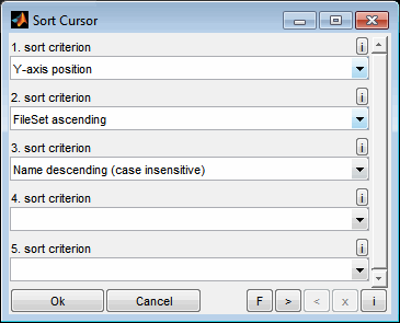
Sort by...

Specify one or more sort criteria (like name, Y-axis position, mean Y-values, FileSet, common Y axis) to sequentially order the cursor channels. This is useful when only one sort criterion does not result in a unique sequence. Criteria related to the values or Y-axis position are considered for the current Y-axis view.

These action changes the cursor order once. Unlike the “Sorted order” option the order is not updated when channels are added.

Mark common Y axes

If activated all channels sharing a common Y axis with the selected channel are displayed with a common marker in front.
Text translation

If the measurement data contains information to translate numerical data to text and this option is activated the cursor will display the text instead of the values. E.g. the display may be “Gear5” instead of 5. This option is also useful in case of a FileSet consisting of multiple files is loaded and the single files should be identified using the channel “FileCnt” (Open / Add / Replace FileSet).
Data tip

Choose to display a data tip near the cursor position while moving the cursor using the mouse or keyboard. The data tip will show axis value of the cursor and the value of the selected channel at the cursor position.
Location inside diagram

Choose to display the cursor text inside the diagram or to place it to the very left side of the window. In the latter case it will overlay with the Y-axis labeling. If the cursor text is displayed on the right and the main view is not indented, the cursor text is displayed independently of the option inside, otherwise it cannot be seen.
Smart update

When this option is activated the numerical values inside the cursor window(s) are only updated when the movement of the cursor line via mouse or keyboard is stopped. Therefore the movement of the cursor line is very smooth even when big data amounts are displayed. On the other hand the values cannot be judged while moving the cursor lines.
Colored decoration

Depending on the stetting the coloration of the channel names and markers is done. No decoration uses no color at all which sppeds up the cursor handling and is recommended in case of many channel names to display. Alternatively only the markers or the markers and the channel names can be colored.
Bold font

Enable to use a bold cursor font.
Contrast scheme

Different color schemes are available to improve the readability especially under dark and bright ambient conditions.
Selected channel indication

The selected channel will be indicated by filling the spaces in the corresponding line with an indication character which is user selectable.

The channel order inside the cursor table can be modified by menu item or keyboard shortcut (Ctrl + Shift + Up / Down). The “Sorted” attribute will be automatically turned off in this case.

If the GPS view is activated all cursor positions are marked there.

The cursor table containing the channel names can be moved vertically using the mouse and between the left and right side by dragging it with the mouse to the other side. You will not see the horizontal movement until you moved the mouse completely to the other side. Additionally the main view can be indented on the left and right end using the mouse to create space for the cursor if these should not overlay the main view. Use the “Location inside diagram” option to determine whether the cursor text is located inside or outside the main view.

8 Marks

Marks define parts of the axis range. They are displayed as green rectangles covering the corresponding axis range in the main view. They are used to define sections for data analysis, saving and optimization. Marks can not overlay.

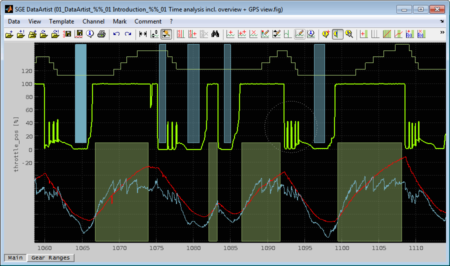
Marks can be created manually or automatically in several ways and using the mouse while Shift-key is pressed.

8.1 Add mark

A mark can be created by entering the x-axis start and end value of the mark (Shift + Ins). Alternatively draw a new mark with the mouse with Shift-key pressed in the main view.

8.2 Delete mark(s)

Marks can be deleted by using the menu item, a keyboard shortcut (Shift + Del) or dragging them outside the main view with the mouse while Shift-key is pressed or by definition of criteria depending on their length and axis positioning (Ctrl + Shift + Del).

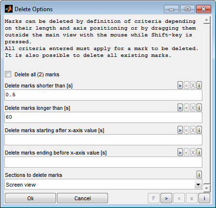
Delete all marks

Check to delete all existing marks ignoring the other criteria below.
Delete marks shorter / longer than

Marks are deleted if they are shorter than this length. Leave empty if criterion does not apply. The range and max. length criterion must also match or be empty.
Delete marks starting / ending before / after x-axis value

Marks are deleted if they are completely located between the "starting" and "ending" x-axis value. Leave empty if criterion does not apply. The length criteria must also match or be empty.
Sections to delete marks

Choose the sections to delete marks from. The mark must be completely within the section for the condition to apply.

8.3 Configure marks

You can configure the marks color and transparency for all or the selected marks (Ctrl + Shift + F4). You can decide whether so save the settings as a global preference.

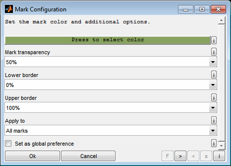
Color

Select the mark color by pressing the button.
Mark transparency

Select the mark transparency level.
Lower border

Select the lower end of the y-axis section to cover by the marks.
Upper border

Select the upper end of the y-axis section to cover by the marks.
Apply to

Select whether to apply the settings to all or the selected marks.
Set as global reference

Select whether to save the settings as a global preference.

8.4 Cut / Extend options

You can modify marks by cutting or extending them (Shift + x).

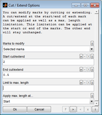
Marks to modify

This option defines the marks to apply the modifications to. This can be all marks, only the selected marks or only the marks at least partly inside the current screen view.
Start cut/extend

This is cut off from every marked section at the beginning. It can be used to remove transient areas at the beginning. If it is negative the mark is extended by this length.
End cut/extend length

This is cut off from every marked section at the end. It can be used to remove transient areas at the end. If it is negative the mark is extended by this length but limited to avoid overlap with the next mark.
Limit length

Marks can be limited to a total maximum length. You can choose whether to apply this change at the beginning or end of the mark with the following option. The other end of the mark will stay unchanged.

This can be used e.g. to cut transient sections at the start of the marks. As is is possible to move the mark borders in both directions it is also possible to completely move a mark by e.g. extending its start and cutting its end by the same value.

8.5 Invert marks

Using this option unmarked sections are marked and the existing marks are deleted.

8.6 Import marks

Marks can be imported from a data file. So if you have the mark start and end axis values in a file you can use this to quickly create marks. This is especially useful to recreate marks that were saved together with data to a file before.

8.7 Automatic mark creation

For all automatic mark creation procedures you can choose in which section you want to work.

Selected / all marks

New marks will only be created inside the already existing marks which will therefore be deleted. This way you can do a step wise mark detection. E.g. you can first set marks to find traction control activation inside a measurement. Then you detect sections inside these marks with specified torque range.
Whole file
Screen view
Unmarked sections

You can also activate a section optimization. See below for details.

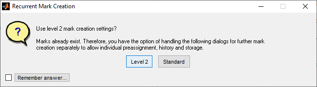
If marks already exist and you start a mark creation again, for some procedures you will be asked if you want to use level 2 settings. In this case the following dialogs for further marker creation will be handled separately to allow individual preassignment, history and storage.

8.7.1 Split equally

Each section to work on will be split equally into a number of new marks (Shift + i).

Zero has a special meaning: The sections are split into the single data points. If a channel is selected its data points will be used. If no channel is selected all data points of all channels will be used. This is e.g. useful if you want every single data point to be used in a optimization separately.

If you have a big number of data points you should turn off drawing marks in this case because it slows down the graphics. See “Section optimization“ for details regarding this option.

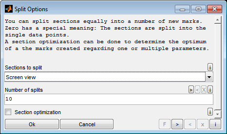
8.7.2 Classify

This method creates marks using a channel and a classes vector (Shift + c). The channel will be used to determine splits when the value of the channel crosses of the classes vector values. So for example you can automatically set marks that classify the measurement into sections of 1000 1/min during an engine speed ramp. Additionally you can use the axis to create classified marks of a specified length.

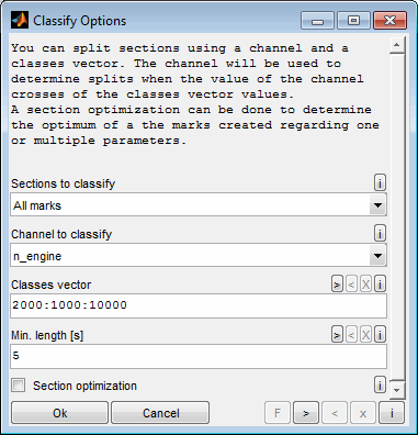
Options:

Sections to classify

Choose the sections to search for ramps or steps. It can be the whole file. Existing marks will be deleted in this case. It can also be all existing marks or only the selected marks.
Channel to classify

Choose the classification channel. This channel will be used to determine split times when the value of the channel crosses of the classes vector values. So for example you can automatically set marks that classify the measurement into sections of 1000 1/min during an engine speed ramp. Additionally you can use the axis to create classified marks of a specified length.
Classes vector

This vector contains the borders of the classes. The vector must be written in valid syntax.

Examples:

"3000 : 1000 : 10000" means from 3000 to 10000 in steps of 1000.

"1000 3000 6000 1000" defines the borders directly.
Min length

To avoid creation of multiple marks at the classes borders due to a toggling signal a minimum demanded mark length can be defined. Marks shorter than this axis length will be skipped.
Section optimization

See “Section optimization“.

8.7.3 Ramp / step detection

You can search areas in the measurement, where a channel has ramp or step characteristic (Shift + r). So for example you can extract the measured ramps in engine bench measurements omitting the warm up and stop engine areas. Or you can analyze ignition sweeps.

If you need more than one channel to identify steps insert a calculated channel that is the sum or product of all needed channels. Factors can help to adjust big differences in signal ranges. A helper function for this case is "multichannel_normalize". It can be passed any number of channels that will get scaled and multiplied. See the SGE_Circus calculated channel documentation for further information.

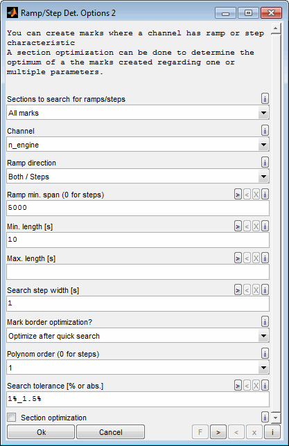
Options:

Sections to search for ramps/steps

Choose the sections to search for ramps or steps. It can be the whole file. Existing marks will be deleted in this case. It can also be all existing marks or only the selected marks.
Channel

Choose the channel to search for ramps or steps.
Ramp direction

Choose the ramp directions that should be searched. In case of step search choose "both".
Ramp min. span

This span between minimum and maximum value a ramp must cross. Leave empty or use zero in case of step search. Value must be positive or zero.
Min. length

Minimum length a ramp/step must last. Value must be positive or zero or empty. Normally the value should be greater than zero to avoid the detection of a big number of zero length marks. Choose the value a little bit smaller than the shortest expected mark.
Max. length

Maximum length a ramp/step may last. Ramps are not cut to this length but discarded if they are longer. Normally this field will stay empty or filled with a value bigger than the longest expected mark. Value must be positive or zero or empty.
Search step width

To speed up detection a quick search is done first. Afterwards the found ramps/steps are corrected with full precision. For the quick search the x-axis step width can be chosen here. It should be at least 5 times smaller than the shortest expected ramp/step. The quick search does not reduce the precision of the data during the ramps/steps. If no step width is used, it is set to zero and the search may be very slow.
Mark border optimization

If you choose no optimization here to save time only the quick search is done. So the marks will only be as exact as the quick search step width.
Polynom order

The order of the polynomial influences the possibility to fit linear or more complex data trends during the ramp. Use 1 for linear ramps and increase if necessary. For step search choose 0. The fitted polynomial for each ramp/step is displayed in the diagram (until the finish message is closed) and helps to adjust the polynomial order.
Search tolerance

It can be relative or absolute. If the value ends with % it is regarded as relative. It is then measured in percent of the mean channel value in the section. This is not suitable for data around zero. If it is a number without % at the end it is interpreted as absolute value measured in the units of the chosen channel. Higher values allow more deviation of the data from the polynomial. Must be >= 0.

Start with small values and increase until all ramps/steps are detected. For step measurement the tolerance must be smaller than half of the step size. Otherwise neighbor steps will not be separated correctly. The tolerance for each ramp/step is displayed in the diagram (until the finish message is closed) and helps to adjust the tolerance parameter and polynomial order. If you encounter problems with separating ramps or steps from the signal jittering using a filtered channel.
Section optimization

See “Section optimization“.

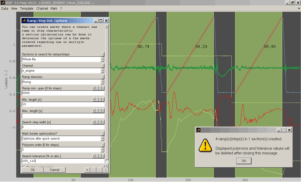
8.7.4 Logical mark detection

You can search in the data for sections where a logical condition is true (Shift + l). Logical mark detection is very fast compared to other methods. Using calculated channels to define the condition enables to perform complex mark detection.

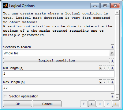
Options:

Sections to search

Choose the sections to search for ramps or steps. It can be the whole file. Existing marks will be deleted in this case. It can also be all existing marks or only the selected marks.
Logical condition

You can modify the logical condition in a graphical manner using the push button. It must only consist of 0 and 1 and must have the dimension of one of the axis vectors. Marks will be created where the condition is true. Using the channel object you can access the loaded channel data.

The following picture gives an example for “Create marks where "B_lamcontrol_enable" is true and "tmot" is below 110”.

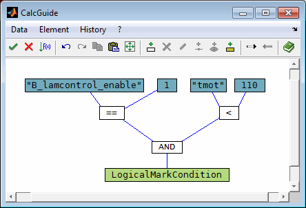
Min. length

To avoid creation of too short marks a minimum demanded mark length can be defined. Marks shorter than this axis length will be skipped. Must be shorter or equal to max. length or empty.
Max. length

Maximum length a ramp/step may last. Ramps are not cut to this length but discarded if they are longer. Normally this field will stay empty or filled with a value bigger than the longest expected mark. Value must be positive or zero or empty.
Section optimization

See “Section optimization“.

8.8 Section optimization

Section optimization can be activated for every automatic mark detection method. This allows to determine the optimum of a section regarding one or multiple parameter channels. In this case the produced marks of a section are regarded as single points and an optimum point is estimated. With this function you can e.g. evaluate ignition sweeps or find the minimum fuel consumption for a operating point depending on injection and cam timing.

The result of a section optimization are then additional channels that contain for every section optimum values (*_opt) for parameter and optimization channel and the fitted values (*_fit) for the optimization channel for every mark. To save the result you can easily mark all optima with a logical condition.

For example to evaluate ignition sweeps the proceeding is the following:

First you do a mark creation (without section optimization) with one mark containing one operating point. So e.g. one mark covers the section of the measurement where engine speed and load are constant. During this section the ignition angle is varied.

Then you start a mark creation in the already existing operating point marks with criteria to mark the single ignition angles. During this mark creation activate the section optimization. Then you are asked to choose the settings for the optimization.

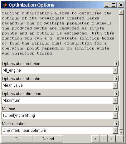
Optimization criterion

Choose the channel to optimize. E.g. torque, fuel consumption or cylinder mean pressure.
Optimization statistic

Choose the statistic calculation for the optimization criterion for each mark. This can be e.g. the mean value if you want to optimize torque or the standard deviation if you want to optimize combustion. Be aware that this is not the optimization direction.
Optimization direction

Which direction is optimum? Do you search the highest or lowest value?
Method

See below for the different method to find the optimum.
Mark creation

You can decide how the marks that are created and used for optimization are kept and displayed. You can keep all marks, no marks or only the nearest mark to optimum. Additionally you can decide to draw one big mark that covers the whole section. The mark creation can be used to influence the data saving behavior. If you choose e.g. statistical calculation you perhaps want the mean value of the channels only near optimum so you decide to keep only the nearest mark. Or you want a stable mean value for the whole section so you decide to draw a big mark for the whole section.

If you are doing an optimization of a big measurement and creating lots of marks during optimization it is useful for runtime and memory usage not to keep all marks but only one per section.

8.8.1 Optimization methods

Different methods to find the optimum are available. These differ in the number of dimensions (= number of parameter channels) and the method used to fit the data and determine the optimum.

1D polynomial fitting

You can choose one parameter channel (e.g. ignition angle). A polynomial curve (order can be chosen) is fitted to describe the relation between the parameter and the optimization channel to find the optimum value for the parameter. A polynomial curve generally does some kind of measure error compensation. This method is only useful if the data shape can be described by a polynomial.

The following additional options are asked for this optimization method:

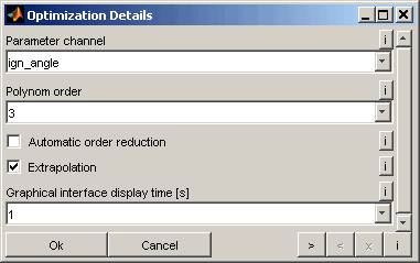
Parameter channel

Choose the channel that is influencing the optimum. This channel will be modified to find the maximum/minimum of the channel to optimize. E.g. the ignition angle in case of ignition sweeps.
Polynomial order

Choose the polynomial order used to fit the data.
Automatic order reduction

If the number of points (=marks) in the section is not sufficient to calculate a polynomial of the demanded order, the order could automatically be reduced. Otherwise the section will be skipped.
Extrapolation

Choose if the fitted polynomial and therefor the optimum can be outside of the measured range (extrapolation).
Graphical interface display time

A graphical interface is available during optimization. Choose the time to display the GUI. 0 means no GUI and "inf" shows the GUI until user input. All other values are times in seconds.

Example "ignition sweeps":

Choose "torque" as optimization channel and "ign_angle" as parameter channel. Then "torque_opt" and "ign_angle_opt" will be created as new channels containing the optimum torque and corresponding ignition angle during the sweeps and NaN otherwise while "torque_fit" contains the fitted polynomial values for each mark. With the logical condition ~isnan("torque_opt") you can easily mark all optima to save them as statistical values.

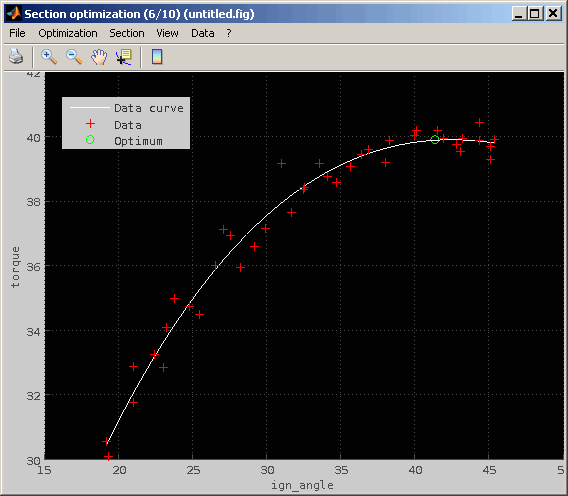
1D cubic interpolation

This method works very similar to "1D polynomial fitting" but instead of the polynomial a cubic curve is used. This is useful if the data behavior cannot be described by a polynomial and has little measurement errors, because the fitted curve will always contain the measured points.

The following additional options are asked for this optimization method:

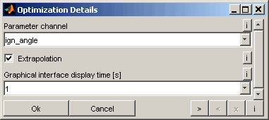
Parameter channel

Choose the channel that is influencing the optimum. This channel will be modified to find the maximum/minimum of the channel to optimize. E.g. the ignition angle in case of ignition sweeps.
Extrapolation

Choose if the fitted polynomial and therefor the optimum can be outside of the measured range (extrapolation).
Graphical interface display time

A graphical interface is available during optimization. Choose the time to display the GUI. 0 means no GUI and "inf" shows the GUI until user input. All other values are times in seconds.

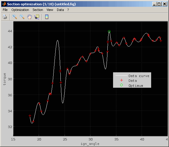
1D simple selection

From the marks of the section the best one is simply selected. No interpolation or fitting is done. Therefore the optimum will always be a member of the created marks and no optimum in between can be found.

The following additional options are asked for this optimization method:

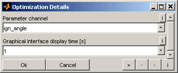
Parameter channel

Choose the channel that is influencing the optimum. This channel will be modified to find the maximum/minimum of the channel to optimize. E.g. the ignition angle in case of ignition sweeps.
Graphical interface display time

A graphical interface is available during optimization. Choose the time to display the GUI. 0 means no GUI and "inf" shows the GUI until user input. All other values are times in seconds.

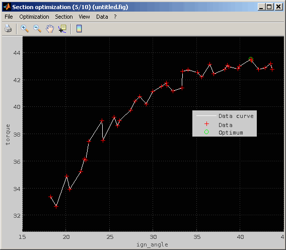
2D map fitting

This method works similar to "1D cubic interpolation" but for two parameters. So two parameter channels are asked and a map is fitted to the data. From this map the optimum is chosen by cubic interpolation. Map creation can be influenced in various ways.

The following additional options are asked for this optimization method:

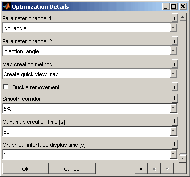
Parameter channel 1

Choose the first channel that is influencing the optimum. This channel will be modified to find the maximum/minimum of the channel to optimize. E.g. the injection timing.
Parameter channel 2

Choose the second channel that is influencing the optimum. E.g. the cam timing.
Map creation method

Choose the method to fit the map. Different methods like quick or optimized maps and planes are available.
Buckle removement

Choose if the fitted map should be smoothed by buckle removal method.
Smooth corridor

Choose if the fitted map should be smoothed by corridor method.
Max. map creation time

Choose the maximum time for map optimization and smoothing (each).
Graphical interface display time

A graphical interface is available during optimization. Choose the time to display the GUI. 0 means no GUI and "inf" shows the GUI until user input. All other values are times in seconds.

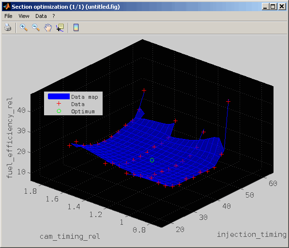
2D simple selection

This method works similar to "1D simple selection" but for two parameters. From the marks of the section the best one is simply selected. No interpolation or fitting is done. Therefore the optimum will always be a member of the created marks and no optimum in between can be found. A map fitted to the data points is displayed but only for visualization.

The following additional options are asked for this optimization method:

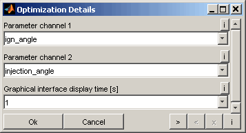
Parameter channel 1

Choose the first channel that is influencing the optimum. This channel will be modified to find the maximum/minimum of the channel to optimize. E.g. the injection timing.
Parameter channel 2

Choose the second channel that is influencing the optimum. E.g. the cam timing.
Graphical interface display time

A graphical interface is available during optimization. Choose the time to display the GUI. 0 means no GUI and "inf" shows the GUI until user input. All other values are times in seconds.

8.8.2 Optimization proceeding

The optimization is done separately for each section the mark creation is done in. Each optimization can be influenced by the user.

Depending on the “Graphical interface display time” setting a window will be shown temporarily for each optimization showing the data, fit and optimum. After the chosen time the window will disappear automatically without interaction. By pressing a key or clicking to the window the automatic proceeding will be disabled.

Using the menu or mouse the following actions can be performed:

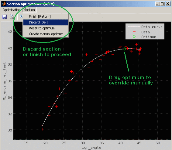
Drag the green optimum circle using the mouse

To override the optimum evaluated by the method chosen just drag the optimum circle using the mouse and proceed choosing by “Section → Finish”.
Section → Finish

Confirm the optimum of the current section shown in the window and proceed to the next section.
Section → Discard

Discard the optimum of the current section shown in the window and proceed to the next section.
Section → Reset to optimum

Reset a manually modified optimum to the one evaluated by the method chosen.
Section → Create manual optimum

Sometimes the automatic optimization may not determine a optimum. In this case the green optimum circle in the window is missing. Using this option a manual optimum will be created and may be modified using the mouse afterwards.
Optimization → Stop optimization

Stop the entire section optimization. A partial result will be preserved.

During optimization the user will be asked whether to automatically save the windows to individual files.

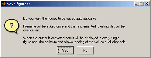
9 Annotations

Annotations enable to highlight and notice events in the data loaded. The visibility of the annotations can be enabled or disabled for all annotations in common (Ctrl+a).

A textual listing of all annotation can be retrieved using the (Data) Info (Ctrl + i).

9.1 Add annotation manually

Different types of annotations are available as well as different reference types of the annotations (Ctrl + Shift + a).

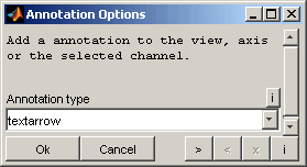
The following figure shows examples of annotations.

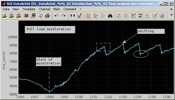
Annotation types

Text arrow

A text arrow contains of a text box and an arrow connected by a line. The position of text box and line can be adjusted using the mouse. The text an some additional properties can be modified to change the appearance.

A text arrow can be linked to a channel or the axis.
Text box

A text box carries some text and has no relation to the channels or axis. The text an some additional properties can be modified to change the appearance.

A text box can only be linked to the window.
Ellipse / Rectangle

A ellipse or rectangle may be used to encircle a section or data event. The background is transparent. A ellipse/rectangle cannot contain any text. The position can be adjusted using the mouse. Some additional properties can be modified to change the appearance.

A text arrow can be linked to a channel, the axis or the window.

Reference types

Reference means that each annotation is linked to either a channel at a specific axis value, or to an axis value independently from a channel or to the window. The reference type essentially influences the behavior of the annotation when e.g. the view is modified (e.g. zoom, axes ranges).

Window

The annotation is linked to the window. Its position will remain unchanged even in case of changing the view by e.g. zooming. The position can be adjusted using the mouse. Window linking is improper to highlight data events or axis points.

Window linking in available for ellipse, rectangle and text box annotations.
Axis

The annotation is linked to the axis. Axis linking is available for text arrows. The arrow is fixed to an axis position and will be automatically kept on that position in case of e.g. zooming. The text position can be adjusted using the mouse.

Axis linking is a proper way to highlight axis points.

When a annotation is added using axis linking the initial position will be retrieved from the cursor if any. Otherwise the mouse position will be used or the middle of the axis if the mouse is outside the window.
Channel

The annotation is linked to a channel at a specific axis position. The annotation is fixed to the channel data value at the axis position and will be automatically kept on that position in case of e.g. zooming or channel range modification. The text position can be adjusted using the mouse.

Channel linking is a proper way to highlight data events. Channel linking in available for ellipse and rectangle annotations.

When a annotation is added using channel linking the initial position will be retrieved from that selected channel at the cursor if any. Otherwise the mouse position will be used or the middle of the axis if the mouse is outside the window.

9.2 Add annotations from file

Annotations can also be created automatically from file events/comments (Alt + Shift + a). Some file formats (e.g. *.mf4) support to store event data. This can be for example trigger events or user pause comments. Depending on the type of event annotations of different types are generated.

In case identical annotations are already exist the annotations to load will be skipped.

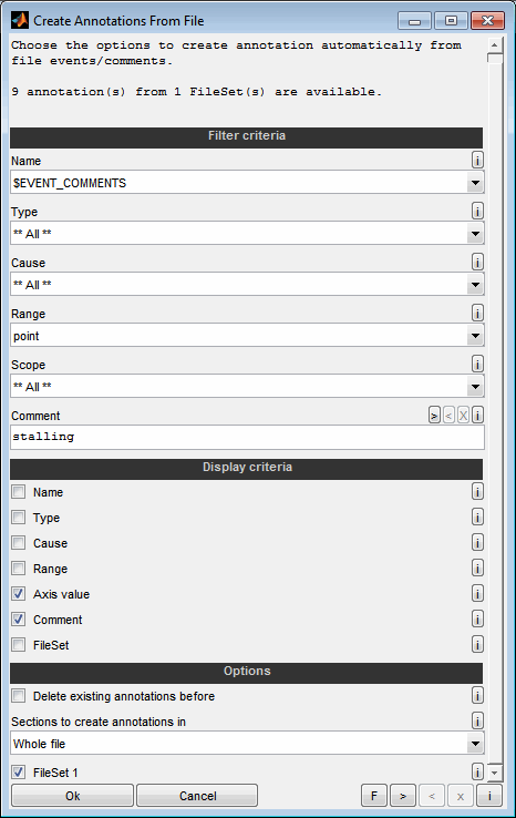
Filter criteria

The filter criteria determine which annotations / events are taken from the files.

Name, Type, Cause, Range, Scope

For each available criterion select the value that must apply for the annotations to load from file. The menus contain all available entries of all loaded files and an entry that includes all options.

Remember that all filter criteria must apply for the annotations to create. The menu contains all available entries of all loaded files and an entry that includes all options.
Comment

Enter a string that must be included in the comment of the annotations to create. Leave empty to not filter depending on the annotations comment. The wildcard * can be used to match any characters. If the string starts with a / the expression will be evaluated as a regular expression.

Remember that all filter criteria must apply for the annotations to create.

Display criteria

The display criteria determine which part of the available attributes is displayed for the annotations that will be loaded from file.

Name, Type, Cause, Range, Axis value, Comment

Select which attributes to show in the annotations textbox.

Options

Choose the sections to create annotations depending on the FileSets and the following axis options:

Whole file
Screen view
All marks (if any)
Selected marks (if any)
Unmarked sections (if any marks)

Additionally you can decide to delete all existing annotations before creating new ones from file.

9.3 Select annotation

The axis range can be adjusted quickly to show one or more specific annotations (Shift + a). Using the corresponding menu item you will be asked to select the annotations to show or search for them.

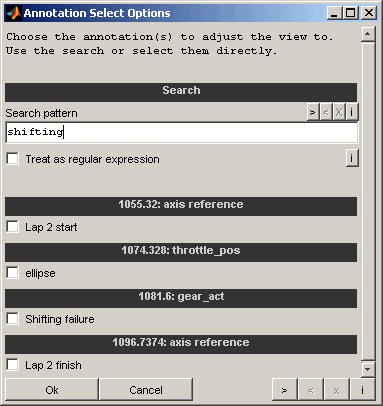
9.4 Delete annotation

Annotations can be deleted using the corresponding menu items or the keyboard if a annotation is selected.

In case of deleting channels the linked annotations will be deleted automatically.

9.5 Edit annotation

Some properties of the annotations can be modified. Using the corresponding menu item or double clicking the annotation leads to a dialog enabling to edit it.

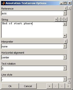
10 Templates

Template files are used to restore data and view configuration efficiently. It is also possible to import *.xda configuration files.

10.1 Save template

Templates are data configuration and view configuration saved to a file. You can save a template from the DataArtist at any time (Shift + s). As this file only contains configuration information it will be much smaller than a session file. But this also means that you need the data files available to load a template. Template files are therefore not useful for data exchange or or long term storage as file path may change.

In case multiple tabs already exist you will be asked which tabs to save.

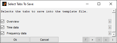
10.2 Load template

You can load a template directly after you started the DataArtist or when you already loaded data (Shift + t). Several options allow you to control the template loading process.

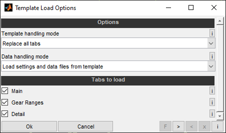
Template handling mode

Decide how to handle the existing tabs when adding new tabs from template.

Replace all tabs

All existing tabs will be discarded before loading the new tabs from template.
Replace active tab

The active tab will be replaced by one one more tabs loaded from template. All other tabs remain unchanged. In this mode exactly one tab must be selected in the bottom section.
Add new tabs

All existing tabs remain unchanged. New tabs loaded from template will be added at the right end.

Data handling mode

Select the content to load from template.

Load settings and data files from template

All data (FileSets and tabs) referenced in the template will be loaded and the template settings like axes ranges and colors will be applied.
Load settings from template, keep data files

Only settings like channels, axes ranges and colors from the template will be applied to the already loaded data (FileSets and tabs). If the template includes more FileSets or tabs that already loaded the missing items will be retrieved from the template.

Load settings from template, ask data files (reference template / loaded data)

All data (FileSets and Tabs) to which the reference refers are queried again and thus other data files to load can be selected. The reference can be the template or the already loaded data. Each FileSet is queried only once. For example, if a set of data files is contained in the first and second FileSet or tab of the reference, they are queried only once and then used in all corresponding FileSets / tabs.

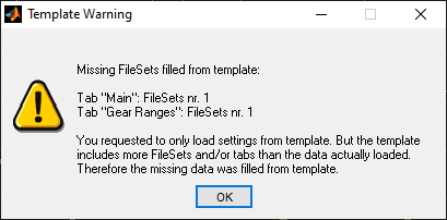
Tabs to load

Select which tab from the template to load. In mode “Replace active tab” exactly one tab must be selected.

To load a template you can choose the file or access recently used templates from the menu directly. When data should be loaded and the data files are not available you will be asked to choose the files manually.

10.3 LastTemplate

Additionally to the manually saved templates a template gets saved every time you exit the DataArtist. These templates are available as “LastTemplate” list. So you can quickly access the configuration used. The name of the template hints to the configuration as it includes the file and channel number and an abbreviated name of the first data file opened.

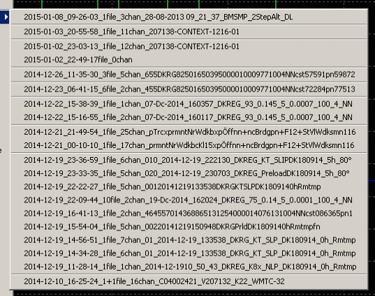
10.4 Cleanup

The list of recently used templates is managed automatically. So entries are automatically removed when the underlying file was deleted. Additionally you can decide to remove entries you don't need any more. You will be asked if you only want to remove the entries or also want to delete the files.

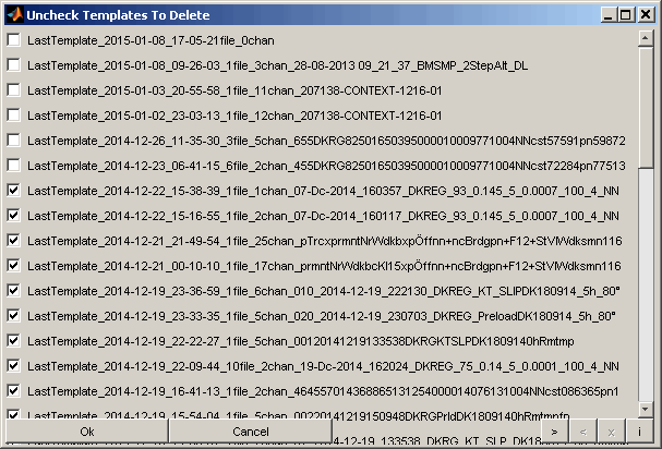
10.5 Restrictions

Some restriction apply when using templates.

When creating channels using the wizard templates saved may not work correctly.
When using xy-view combined with calculated channels templates saved may not work correctly.

Generally it is recommended to test loading a saved template before the source window is closed if you use not standard configuration. In case of problems you can always save a session file.

11 Save data

11.1 Save session

The whole session including data can be stored as file (Ctrl + Shift + s). After re-opening the whole functionality can be used again immediately. Sessions also work with xy-view, wizard channels and special channel configuration (e.g. marker).

Session files can be opened the same way as data files or using the SGE Viewer.

Session files may get very large as they contain the loaded data. Consider using templates if you want to make views and setting available. But remember that using templates brings some restrictions. See the template section for details.

11.2 Save to file

You can use the DataArtist not only to view data. You can also save data to one or multiple files (Ctrl + s).

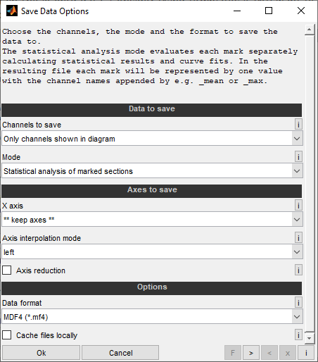
Channels to save

This may be the already loaded channels from the display. Or all channels that the loaded file(s) contain. This is a convenient method to quickly arrange the data section to save with only some channels loaded and then to save all channels from file without displaying them. It is also possible to do a manual selection of the channels to save. In case multiple FileSets are loaded the channels to save will be asked for each FileSet sequentially.
Mode

Several possibilities to define the axis range and mode of the data to save are available.
- Whole loaded file
  
  The entire data loaded will be saved.
- Screen view
  
  The data section of the actual view will be saved.
- Marked sections to file
  
  If the sections to save are based on existing marks you can save them to one or multiple files. In case of multiple files the first file name is asked and all other file names are based on the first one including a counter. When saving to one file the axis could be shrinked to have the data concatenated in the new file. Otherwise the unmarked section will appear in the new file without values.
- Statistical analysis
  
  This is a special mode that evaluates each mark separately calculating statistical results. So in the resulting file for each mark will appear one value. The channel name is appended with a string indication the statistical calculation like “_mean” or “_max”. Additionally to the standard statistical calculations curve fits (exponential, polynomial) are available.
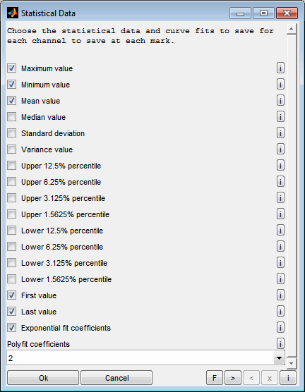
X axis

Select which axes the stored data should have. You can either keep the axes unchanged or interpolate all data to a common X-axis. This new axis can be either that of a loaded channel or the total number of axes of all channels to be saved. Double points are removed to obtain a strictly monotonous axis. Therefore, the order of the axes in the stored data may differ from the displayed data.

The calculation is performed only for the data to be stored. The loaded data will not be changed.

Some data format (like spreadsheet and csv) require a common axis. For these formats this options will be activated automatically even if "keep" is selected.
Axis interpolation mode

Select the interpolation mode to use when channels need to be interpolated to new axes.
- left: Look for the next value of the affected channels to the left axis side. In this way, only values that are actually contained in the data can be created. However, the data can be "old".
- linear: Perform an linear interpolation of the affected channels. This can result in intermediate values that are not contained in the loaded data.
Axis reduction

If this option is active, only the data points that change are stored for the channels to be saved. As long as a channel has a constant value, these points are removed.

This reduces the file size, but changes the data. Decide whether they value file size or unchanged data. This option can only be used for MDF3/MDF4 target formats and not for statistical data.
Data format

The data can be saved in different formats.
- MDF3 (*.dat)
- MDF4 (*.mf4) uncompressed / compressed
- Ascii (*.csv)
- MATLAB (*.mat)
- OpenOffice (*.ods), when Apache OpenOffice is installed.
- Excel (*.xls), when Microsoft Excel or Apache OpenOffice is installed.
- Google Maps/Earth import file (*.kml)
  
  This format allows you to import the data into Google Maps/Earth. This allows you to display the data geographically. In addition, it is possible to visualize the loaded data. In this way any measurement data can be displayed geographically.
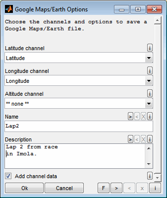
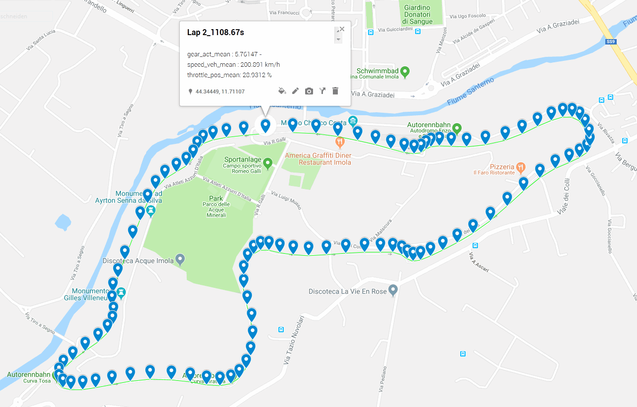
Cache files locally

Create file(s) locally first for performance reason. If this option is selected the files will be created in a local temporary directory first and copied to the final destination afterwards. Use this option if you experience slow performance writing to network files.

11.3 Copy (to clipboard)

Data can be transferred comfortably to the clipboard or an external text editor (Ctrl + c). In this way, parts of the data can be made visible very quickly or used outside the software. The format of the clipboard content is configurable will be suitable to paste into a spreadsheet software.

Copying big amounts of data may last long and exceed the capabilities available.

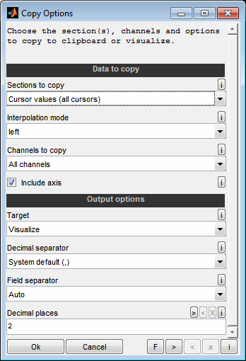
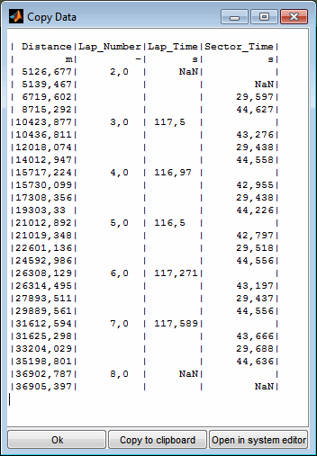
Sections to copy

Choose the sections to copy the data to clipboard from.

Whole file
Screen view
All marks (if any)
Selected marks (if any)
Unmarked sections (if any marks)
Cursor values (if any)

Interpolation mode

At the axis positions to copy some channels may not contain values. This might happen e.g. because of different data acquisition rates. You can decide how to proceed in this case.

None: Do not fill missing values automatically. Affected channels or axis positions will be missing in the copied data.
Left: Look for the next value of the affected channels to the left axis side. In this way, only values that are actually contained in the data can be created. However, the data can be "old".
Linear: Perform an linear interpolation of the affected channels. This can result in intermediate values that are not contained in the loaded data.

Target

Select the target for the copied data. It can be the system clipboard or a visualization that enables to view the data and to open it in an external editor.
Decimal separator

Choose the decimal separator for numbers to use when copying.
Field separator

Choose the field separator to use when copying. Use "Auto" for automatic detection depending on "Target".
Decimal places

Enter the maximum number of decimal places to use. Leave empty to detect automatically.

12 Present, print, organize

12.1 Copy to clipboard, print

Analyzing data often includes the need to present the results. Therefore the DataArtist makes it available to export the actual view into the clipboard or file formatted in a way that is suitable to be useful for different targets (Ctrl + shift + c).

Document
Email
File
Printer

This can be different sizes of clipboard content. "Email" and "Document" are specially sized to fit into a email or document software. "Email" creates a bitmap format while "Document" creates a vector format. Some paper formats are also available and all windows can be printed and saved to file in various formats.

The created window is configurable. So you can move elements like legend or cursor boxes. It is also possible to add lines, arrows, text boxes etc. to the window to explain or highlight.

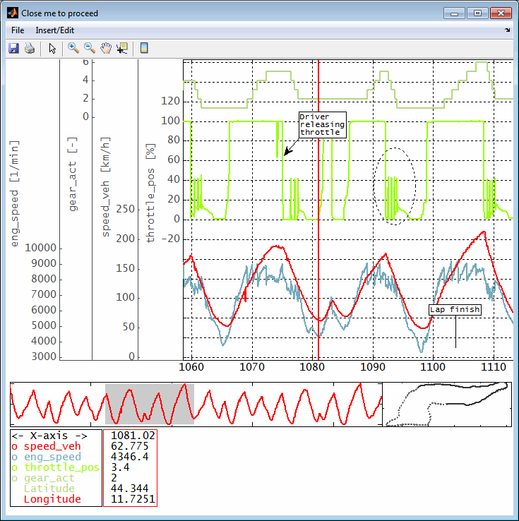
During creation some options will be asked to define the base layout of the window.

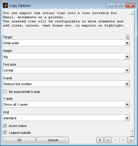
After closing the window the content will be copied to clipboard and can be pasted / used in the target software.

12.2 Window handling

Since the SGE Circus offers to open a considerable number of windows an automatic window handling feature is implemented. Using the corresponding menu item enables to arrange all or a subset of the windows of the current session.

Close windows

This feature enables to close visible and invisible windows automatically.

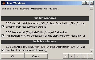
Windows

Select which windows to close. The windows will be closed without saving anything and without any further confirmation. Visible and invisible windows will be listed separately.

Resize windows

This feature enables to automatically set windows to fixed sizes or to maximize, minimize and restore them.

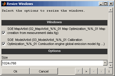
Windows

Select which windows to resize.
Size

Select the desired window size. It is possible to maximize, minimize and restore windows. Additionally a set of fixed standard sizes are available.

Arrange windows

This feature enables to automatically arrange windows.

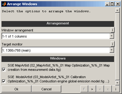
Window arrangement

Select the layout of the arrangement. It is possible to maximize, minimize, restore or close all selected windows. Additionally column and row based layouts are available.

Example: "2-3 of 5 rows" means that the screen is split into 5 rows and the second and third row is used for the layout.
Target monitor

Select the target monitor for the windows to arrange in case of multiple monitors are connected to the computer.
Windows

Select which windows to include into the arrangement.

Toggle windows periodically

This feature enables to automatically toggle windows to create kind of a movie. This can be used to compare windows.

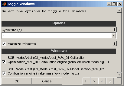
Cycle time

Select the the time to wait before activating the next window.
Maximize windows

If enabled the windows will be maximized before toggle to ensure identical size.
Windows

Select which windows to toggle periodically.

13 General information

Duplication, processing, distribution or any form of commercialization of the documents content beyond the scope of the copyright law shall require the prior written consent of the SGE Ingenieur GmbH. All trade and product names given in this document may also be legally protected even without special labeling (e.g. as a trademark).

MATLAB, Simulink and Stateflow are registered trademarks of The MathWorks Inc., Natick, MA, USA.
Microsoft, Microsoft Windows and Excel are either registered trademarks or trademarks of Microsoft Corporation in the United States and/or other countries.
Apache and OpenOffice are trademarks of The Apache Software Foundation.

The SGE Circus includes Third Party Software. For details please refer to the → SGE Circus documentation.

SGE Ingenieur GmbH – www.sge-ing.de

Contents

1 Introduction

1.1 SGE Circus user manual

1.2 SGE CalcGuide user manual

1.3 SGE Circus videos (external)

2 Keyboard shortcuts, mouse gestures

3 Features

4 Data handling

4.1 Open / Add / Replace FileSet

4.2 Delete FileSet

4.3 Drag and drop, paste clipboard

4.4 File update

4.5 Check files

4.6 Delete data

4.7 (Data) Info

4.8 View / edit comment

5 Channels

5.1 Add / Delete

5.2 Select / Search channel

5.3 Channel configuration

5.4 Color

5.5 Range

5.6 Show / hide

5.7 Shift

5.8 Style channels automatically

5.9 Channel info

5.10 Rename

5.11 Channel wizard

5.12 Analyze

5.12.1 Histogram

5.12.2 FFT

5.12.3 MapArtist

5.13 Show calculated channels

5.14 Split channels

5.15 Reduce data

5.16 Create mark indication channel

6 View

6.1 Main view

6.2 Overview

6.3 GPS view

6.3.1 GPS lap step click

6.3.2 Overview / GPS options

6.4 Tabs

6.5 Snapshot

7 Cursors

8 Marks

8.1 Add mark

8.2 Delete mark(s)

8.3 Configure marks

8.4 Cut / Extend options

8.5 Invert marks

8.6 Import marks

8.7 Automatic mark creation

8.7.1 Split equally

8.7.2 Classify

8.7.3 Ramp / step detection

8.7.4 Logical mark detection

8.8 Section optimization

8.8.1 Optimization methods

8.8.2 Optimization proceeding

9 Annotations

9.1 Add annotation manually

9.2 Add annotations from file

9.3 Select annotation

9.4 Delete annotation

9.5 Edit annotation

10 Templates

10.1 Save template

10.2 Load template

10.3 LastTemplate

10.4 Cleanup

10.5 Restrictions

11 Save data

11.1 Save session

11.2 Save to file

11.3 Copy (to clipboard)

12 Present, print, organize

12.1 Copy to clipboard, print

12.2 Window handling

13 General information