SGE MapArtist – User Manual

www.sge-ing.de – Version 1.62.67 (2022-07-24 22:21)

1 Introduction

The SGE MapArtist is a tool for ECU map creation, visualization and optimization. This manual gives information about the topics regarding the SGE MapArtist only. The SGE MapArtist is part of the SGE Circus. For help topics regarding general features please refer to the corresponding documentation accessible using the links below.

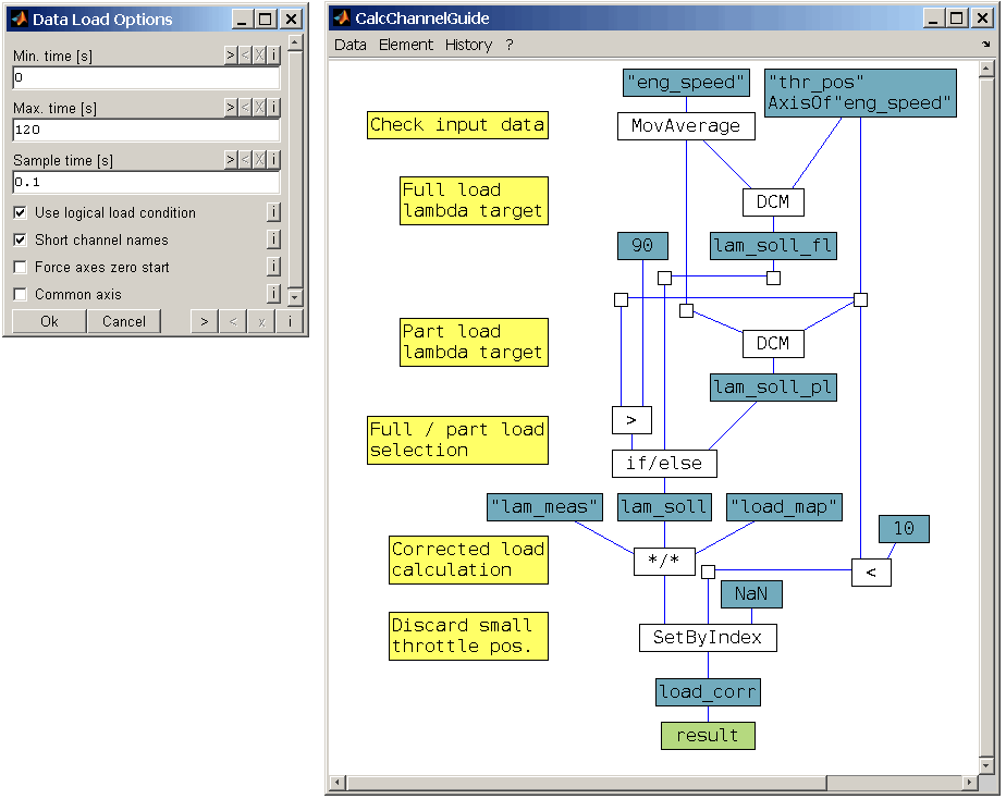
1.1 SGE Circus user manual The SGE Circus documentation makes available general information regarding data loading procedure, input handling, preferences, history and other topics concerning all tools.	1.2 SGE CalcGuide user manual The SGE CalcGuide is a tool to implement calculation routines by creating graphical flow chart diagrams - included with all tools.

1.3 SGE Circus videos (external) Videos and tutorials are available on the internet.

For information regarding the version dependent software changes please refer to the Release notes accessible using the corresponding menu item inside the SGE Circus.

2 Keyboard shortcuts, mouse gestures

Many functions are quickly accessible via keyboard shortcuts. For a list of available keyboard shortcuts, see the list below. In addition, the entries in the menus and context menus as well as the tooltips of the toolbar point to shortcuts.

Map Handling
Ctrl + t	Load maps / axes...
Ctrl + s	Save calibration parameter file / send map to INCA ...
F4	Map Configuration
Shift + 1..6	Select active map
Ctrl + Shift + 1..6	Toggle map visibility
Shift + del	Delete map...
Shift + l	Toggle legend visibility
Ctrl + Shift + Up/Down	Change map order in legend
Data Points Handling
Ctrl + o	Load data points...
Ctrl + d	Delete data points...
Ctrl + Enter	Data color / description ...
View
Ctrl + 1	Activate 1D view. Toggle modes in 1D: value, value+diff, value+diffrel, diff, diffrel
Ctrl + 2	Activate 2D view. Swap x/y in 2D view.
Ctrl + 3	Activate 3D view.
Ctrl + 5	Activate 2D+3D view. Swap x/y 2D+3D view.
Ctrl + Arrow (only 3D) Mouse button Ctrl / Shift + mouse wheel	Rotate
Ctrl + + / - Ctrl + Arrow (only 2D) Mouse wheel	Zoom
Ctrl + r Ctrl + F12	Toggle standard views, reset axes (2D/3D). Modify table width (table view).
Shift + Mouse button twice	Center map at marked point (marked points must stay) / Extend marked map points
Ctrl + Mouse button, Ctrl +Mouse move	Add to / Remove from marked map points
Shift + r Shift + F12	Toggle standard views, keep axes
Ctrl + Shift + / -	Increase / decrease data display reduction
Ctrl + Shift + F12	Automatic data display reduction
F8	Toggle active page (working / reference) page
Ctrl + F8	Toggle visibility of background reference page
Ctrl + p	Toggle data point visibility
Ctrl + l	Toggle error lines point visibility
Ctrl + m	Toggle map visibility
Ctrl + e	Toggle error map visibility
Shift + enter	Color map...
n	Next color
Ctrl + n	Previous color
Ctrl + a	Mark all map points (2D, 3D). Toggle mark all, map, axes (table view).
Shift + n	Toggle number of lines in 2D view
Shift + l	Toggle legend visibility
Ctrl + x	Set axes ranges or set axes tick to accord with map breakpoints...
Map Calculation
Shift + c	Calculate / optimize map...
Shift + s	Smooth map...
Shift + a	Optimize axes...
Map Editing
+ * / =	Modify by calculation / set value...
-, 0..9	Start direct value input...
space, F2	Set value (only table mode)
(Ctrl +) (Shift +) F7/F6 Ctrl + Shift + mouse wheel	Increment / decrement
Ctrl + c / v Ctrl + Shift + v	Copy / paste data to / from clipboard. Paste using operations (+,-,*,/). Additionally it is possible to paste files or strings containing file names to the present to load maps or data points.
Shift + w	Copy map+axes...
Ctrl + u	Reset value to reference page
Ctrl + Shift + f	Copy working page to reference page
Shift + m	Mark map by condition...
Ctrl + k	Conversion rule settings...
Shift + k	Apply conversion rule
Advanced Editing
Shift + x / y	Interpolate
Ctrl + Shift + x / y	Distribute changes
Ctrl + Shift + e	Extrapolate...
Ctrl + g	Limit gradient...
Shift + Mouse button	Move axis breakpoint in 3D view (mark and unsnap first)
Miscellaneous
F1	Show manual...
Shift+F1	Show keyboard shortcut manual...
Ctrl + z	Undo (views, marks)
Ctrl + y	Redo (views, marks)
Ctrl + Shift + c	Copy window to clipboard..., Print window...
Ctrl + Shift + s	Save session...
Ctrl + Shift + i	Data info...

3 Features

The main features of the SGE MapArtist are listed in this introduction. For details please see the following sections.

Data Import Measurement Points

Formats MDF3/4, ASCII, Diadem, FAMOS, Horiba-VTS, IFile, Kistler *.ifi, BLF/ASC CAN files, Excel*, OpenOffice*, MATLAB, Magneti Marelli, MoTeC, 2D-Logger, Get-Logger, Tellert, Keihin (* if Apache OpenOffice or Microsoft Excel is installed)
Data import from MATLAB workspace, function calls, Simulink simulations and DLL output
Any number of files can be loaded
Down-sampling and time period freely selectable
Loaded data can be filtered by any logical expression
Definition of any calculated channels including features like map interpolation and Simulink systems integration. By direct use of filters and calculations, the pre-processing of data can often be eliminated.

Data Import Maps, Axes

Sources
- DCM-, PaCo-, CDFX-files
- ETAS INCA software
- Mectronik MeCal files (*.rbe, *.rbs, *.apu, *.rex, *.mke)
- BMW Race Calibration files (*.bmwrc*)
- From clipboard with/without axes (e.g. from INCA, Excel, OpenOffice)
- From other MapArtist sessions
- Creation (incl. automatic axes generation)
Consideration of axes groups, units, increments
Transposition possible
Any number of maps can be loaded simultaneously

Map Export

DCM-, CDFX-files
Direct transfer to INCA (*) via COM interface
Mectronik MeCal files (*.rbe, *.rbs, *.apu, *.rex, *.mke)
MATLAB script (*.m)
Data exchange using cliboard (single points, sections, map with/without axes)

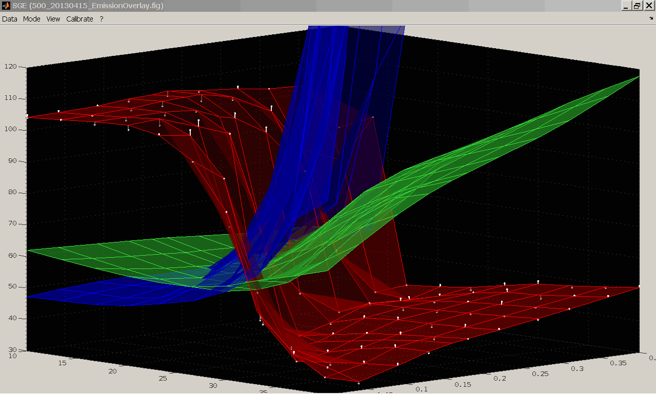
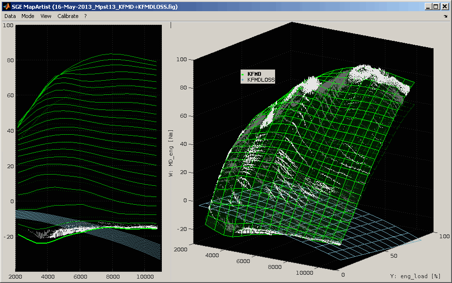
Map Display

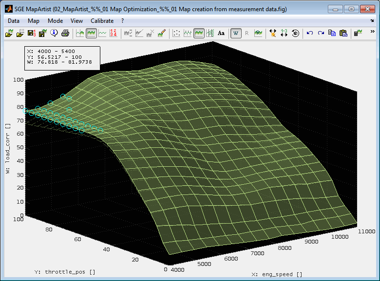
3D-Map / Iso-Diagram
- Display of map, data points, error lines (individually detachable)
- Colors, transparency, lines, points, light source configurable
- Rotate, zoom with automatic down-sampling for flowing display even of large amounts of data
2D-Lines
- Display of 1/3/all map-lines, data points, error lines (individually detachable)
- Display via x- or y-axis
- Automatic or manual zoom and Pan

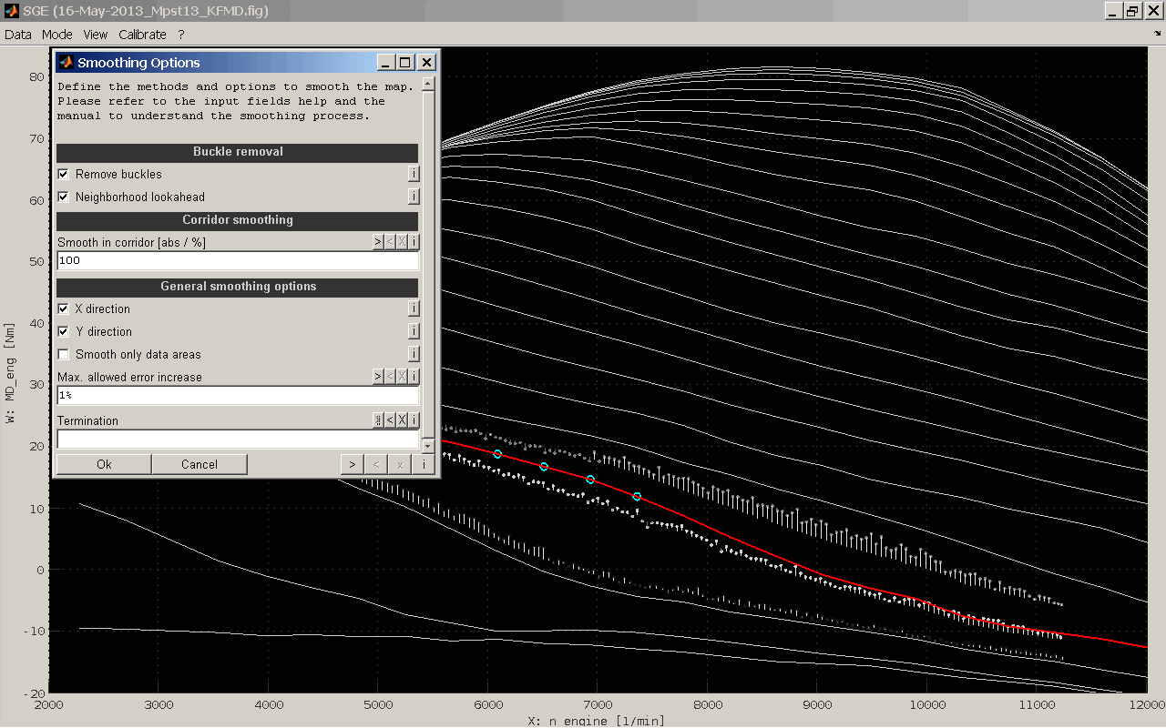
Table View
- Differences working/reference page are displayed in terms of color
- Data exchange via clipboard
- Axes can be edited comfortably, since monotony is only checked when the view is exited

Map Creation

Automatic map optimization
- Quick view
- Map optimization (data mean value, above data, below data)
- Gaussian Process Model
- Fit plane, fit polynomial 2nd/3rd order
Automatic map smoothing
- Several smoothing algorithms
- Definable boundaries for values and error
- x-/y-direction selectable separately or together
Automatic axes optimization
- Areas definable
- x-/y-direction selectable separately or together

Map Editing

Working / Reference page
Increment, decrement, +, -, *, /, %
Set to reference page value
Interpolating, extrapolating
Distribute changes

Cursor

Displays the current point or current range if multiple points are selected
Difference Working / Reference page
Absolute / relative error referenced to data points
Mark color shows improvement / deterioration during adjustment

Session

The whole session including data can be stored.
After re-opening the whole functionality can be used again immediately.
File size depending on loaded data.

History

Undo- / Redo-functionality
All dialog have a history and filters to find former inputs quickly.
All dialog offer export and import functionality to load and document inputs.

Info

Display information about loaded data, data files, time ranges, calculated channels and measurement comments
Information about the origin of template and map(s), size and axes
Map history
Documentation and validation

Graphic Export

Configurable export of the actual screen to the clipboard
Ready formatted for email or office software. Reports made easy.
Axes, fonts, sizes, adjustable. Adding notes, highlights, etc.

Data Exchange

Copy / Paste of data to / from the clipboard to 2D/3D and table view
Print window

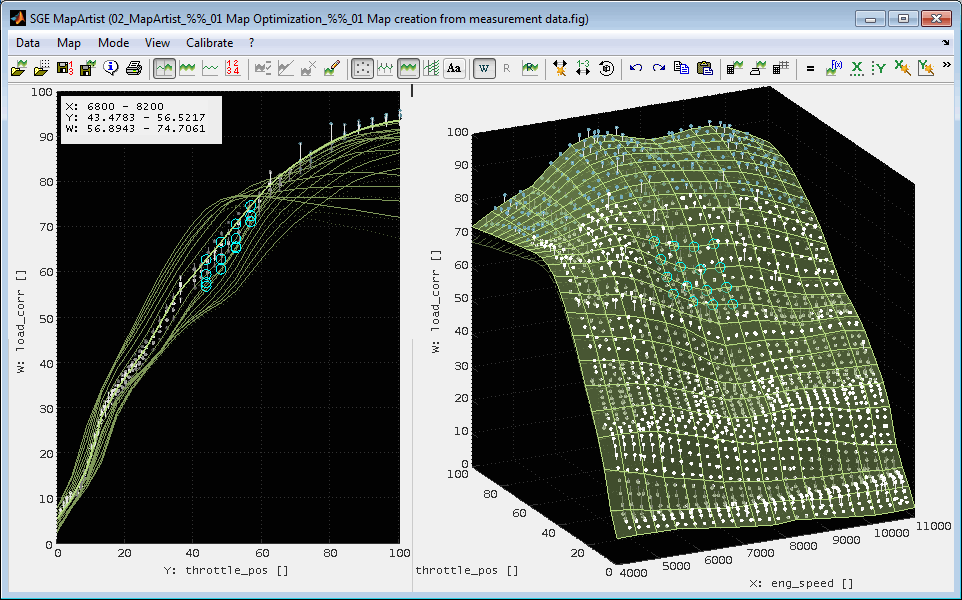
4 Map(s)

4.1 Map handling

The main purpose of the MapArtist is to create, visualize and optimize maps. Therefore any number of maps can be loaded or created simultaneously.

Exactly one of the loaded maps will be the active map at a time. Only the active map is fully functional. All other maps are just displayed in standard manner. So e.g. only the active map can be edited, marked and copied. Error maps, error lines and iso-contour plots are only available for the active map.

A legend can be displayed (Ctrl + l) to identify the active and loaded maps as well as the data point sets. In table view a tooltip will be shown to identify the active map when the mouse rests on the table.

The main map handling operations are:

Add maps

Additional maps can be loaded or created (Ctrl + t). See the following section for details.
Duplicate map

Maps can be duplicated to handle them separately. A counter will be added to the name of the new map.
Delete map

Loaded maps can be deleted if at least one map remains (Shift + del).
Select active map

The active map can be selected from the loaded maps (Shift + 1..6). This can also be done using the menu or double clicking the corresponding legend entry. Data relating to the map is restored when a map is made inactive and active again later on. So e.g. the undo history is selective for the single maps.
Toggle map visibility

The visibility of single maps can be toggled if they are not the active map (Ctrl + Shift + 1..6). The visibility of the active map and e.g. the data points and error lines are modified separately using the “View” menu item or keyboard shortcuts.
Change map order

The order of the maps shown in the legend can be modified (Ctrl + Shift + Up/Down).

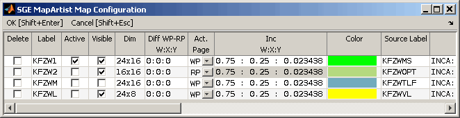
Additionally to using keyboard shortcuts or the menu items most map handling and configuration operations can be performed using the Map Configuration utility (F4).

4.2 Working page / reference page

The active map is available as reference and working page. Either the working or reference page can be activated (F8). Additionally the reference page can be made visible while the working page is active (Ctrl + F8). The reference page map is displayed using a dotted line.

The working page can be edited. The reference page is write protected. The only ways to modify it is to save the working page as reference page (Ctrl + Shift + f) or to load a new template map with different axes size (Ctrl + t). In this case the template is also loaded to the reference page to keep the dimension of reference and working page map identical.

You can also copy the reference page to the working page.

4.3 Load / replace template maps

Templates are maps and their axes. They can be displayed, compared, changed and saved again. Templates must have strictly monotonically increasing axes. The axes are automatically adjusted if they do not meet the condition.

Several sources are available to load template maps from. It is also possible to create a new map without using any external source. See the following section for a description of all template generation options.

When you load a template map (Ctrl + t) for the first time during a MapArtist session it is made the active map and working and reference page are initialized with the template map data.

When you reload a template map (Ctrl + t) different modes are available to add or replace maps or to interpolate maps to new axes. See below for a description of all template load modes.

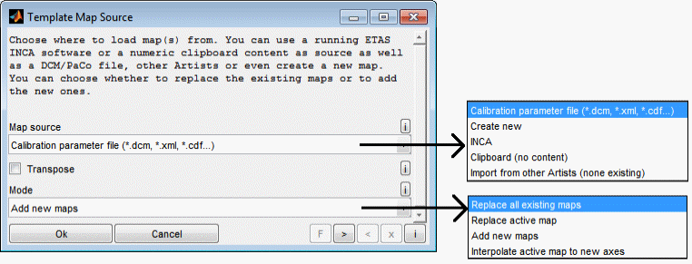
4.3.1 Map sources

DCM / PaCo / CDF - file

You can load the template map from a DCM, PaCo or CDF file. The file will be asked and you can choose from all map labels in the file. In addition to using the file load dialog, you can load sessions and template data files by using drag and drop or the clipboard. To do this, one or more files can be dragged directly to a MapArtist session or inserted via keyboard shortcut (Ctrl + c / v). It is also possible to copy files directly to the clipboard as well as strings containing the file names line by line.
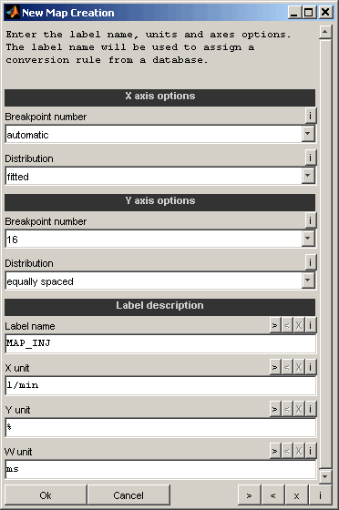
Create new

You can create a new template map without using any external source.

The map will be initialized with zero values. The map size, distribution type, name and units can be defined.

If data points were loaded you can choose "automatic" to get the breakpoint number and values determined automatically to match the data. The distribution can be equally spaced or fitted to the data if any data points were loaded.

The name must consist of a-zA-Z0-9[]_. only with a max. length of 1024 char and must not start with a digit. The label name will be used to assign a conversion rule from a database. So make sure to use the exact label name here in case of creating a label to later transfer to a system using conversion rules (e.g. ECU).

INCA

A map can be retrieved from ETAS INCA software. Therefore INCA must be started and an experiment must be opened. The map will be retrieved from the active calibration page. If you get the map from INCA also A2L information (conversion rule) is collected. This will be used in case the map is saved as DCM later to use the correct group axes, units and to define the conversion rule used while editing the map, e.g. the increment used for incrementation.
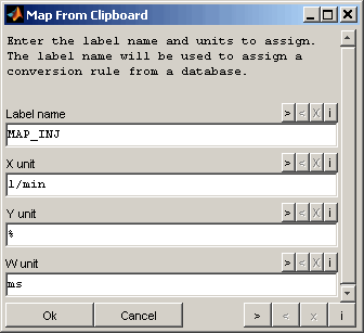
Clipboard

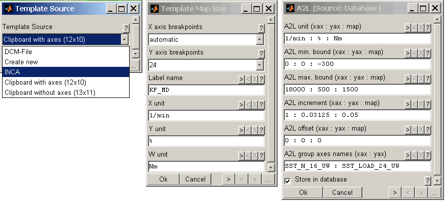
If you copied a map to clipboard this data can also be used to create a template. The clipboard data can be with or without axes. When no axes are loaded they are created as integer vectors starting at one. Sources for suitable clipboard content are spreadsheet software or calibration software like ETAS INCA (→ Copy all data to clipboard) or MoTeC (→ Export To Clipboard, CSV file).

Import from other Artists

You have the possibility to import maps from other currently opened MapArtists. The maps must be visible in 3D mode. A list of all available maps will be shown afterwards to select the ones to import. If you miss maps to import make sure they are shown in 3D mode in the other MapArtists.

In standard mode the maps will be imported using the color from the source MapArtist. Using the corresponding option you can automatically assign colors not yet in use for the imported maps.

Additionally you have the option to close the source MapArtist windows after import. Make sure to save the work before deciding to do so because the windows will be closed without conformation.
Other maps

In case of interpolating the active map to other axes these can be retrieved from other loaded maps directly.

4.3.2 Modes

Replace all existing maps

All existing maps in the MapArtist will be deleted before loading the new template maps.

Any number of template maps can be loaded simultaneously in this mode.

Replace active map

The working page of the active map will be replaced by the template map to load. If the dimension of the new template map differs from the dimension of the active map, also the reference page will be replaced to assure equal dimensions.

Exactly one template map must be loaded in this mode.
Add new maps

All existing maps in the MapArtist are kept while loading the new template maps. If any of the new label names/sources overlaps with an existing their names will be appended with a counter automatically.

Any number of template maps can be loaded simultaneously in this mode.
Interpolate active map to new axes

The working page of the active map will be interpolated to the axes of the template map to load. The values of the map to load are irrelevant in this case - only the axes data will re regarded. If the dimension of the new template map differs from the dimension of the active map, also the reference page will be replaced to assure equal dimensions.

Exactly one template map must be loaded in this mode.

4.3.3 Transpose

You can choose to transpose the template map to load. In this case the x- and y-axes are swapped also. This option is only valid when loading a template from any source. It is ignored when creating a new template.

No A2L information will be retrieved in this case.

4.4 Save maps

Different targets are available to export the active map to. These are file formats like DCM/CDFX and CSV file (suitable to import into MoTeC software), MATLAB scripts (*.m) as well as direct transfer to ETAS INCA software. Of course data can alsi be transferred using the clipboard.

If, when loading the template maps, they were automatically adjusted to have strictly monotonically rising axes, these modified axes are also used when saving. In case the map to save to DCM/CSV file or ETAS INCA software contains invalid values (NaN) you will be asked for a replacement value. Leave empty to keep the invalid values.

4.4.1 Save calibration parameter file

The working page label can be saved as calibration parameter file (*.dcm, *.cdfx, *.dcmap, *.csv, *.m) (Ctrl + s). The *.m format supports to generate a MATLAB script file to transfer the calibration parameters into the MATLAB/Simulink workspace. The CSV file has a format suitable to import into MoTeC calibration software. Choose whether to include the complete comment from the "Data → Info" as label "Comment" into the file.

You can enter an extra comment here that is additionally saved as label "Comment" to the file. Select the name for the label to create and to save into the file. Default is the name of the loaded template label.

Several A2L options are asked when saving to calibration parameter file and “Apply A2L settings” is checked . This is needed if the file should be conform to the description file of the ECU. The correct group axes are especially important, because otherwise the axes will not be loaded by the calibration software even if they are saved with the map. The values are prefilled if this information is available for the label name. They will be retrieved when loading a template map from ETAS INCA software or from an internal database. Therefore it is especially important to set the correct label name in the options dialog.

Even if you decide not to apply the “Apply A2L settings” any group axes information available (e.g. if label was loaded from calibration parameter file) will be maintained and transferred to the new file to save.

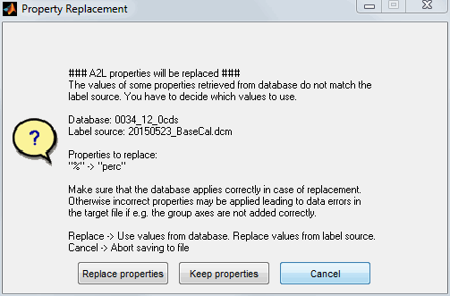
If the information from this dialogue does not match the information already linked to the map you will retrieve a warning to confirm the replacement of the properties. This may for example happen if you load a template map from a calibration parameter file while the previous dialog is filled from the database or if you choose to save to a different label name. If the project of the label in the database does not match the one of the calibration parameter file, some properties may be different. It is important to check the properties to replace because otherwise data errors in the file may happen by applying wrong properties like group axes.

4.4.2 Save as MATLAB script

A map can be saved as a MATLAB script (*.m). When this script is executed in MATLAB, the map and its axes are created in MATLAB workspace and are available for calculations and simulation in MATLAB and Simulink.

The following options are requested in this case:

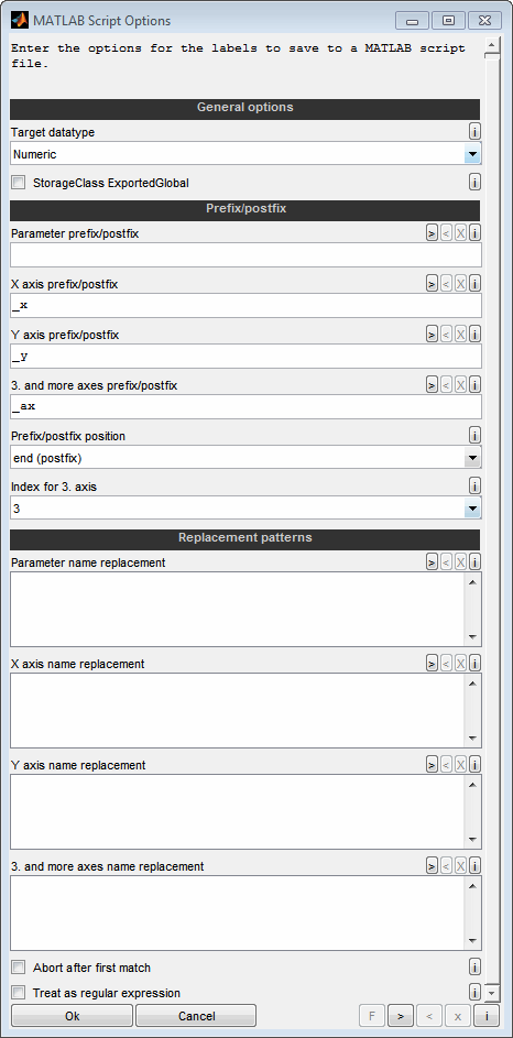
Target datatype

Decide whether you want to generate the parameters as numeric variables (e.g. scalar, curve, map) or as Simulink.Parameter type.
StorageClass ExportedGlobal

Decide whether you want to set the storage class for the created parameters to ExportedGlobal. This is only possible for Simulink.Parameter type.
Parameter prefix/postfix

You can append any text before or after the name of the parameter. Basis is the name as it was loaded in CompareArtist. Typically this field is empty to not change the name.
X/Y prefix/postfix

You can append any text before or after the name of the X/Y axis. Basis is the name as it was loaded in CompareArtist. This field typically should not be empty to make sure to have an individual axis name differing from the prameter name.

Example:

"_x"
3. and more axes prefix/postfix

You can append any text before or after the name of the 3. and more axes. Immediately after this text, a number is automatically appended which represents the number of the axis. The number depends on the following settings. This field typically should not be empty to make sure to have individual axes names differing from the parameter name.

Example:

"_ax" will lead to _ax1, _ax2...
Prefix/postfix position

You can append any text before or after the name of the parameter. Immediately after this text, a number is automatically appended which represents the number of the axis. The number depends on the following setting.
Index for 3. axis

For the third and following axes, a number is automatically appended to the text of the previous setting. Decide here which number is used for the third axis. All following axes will then have correspondingly higher numbers.
Parameter / axis name replacement

You can use replacement rules for the parameter names. One rule per line. The string to look for and the replacement are separated by two colons, like "Map :: Table". The replacement is case sensitive, done in the order of lines from top to bottom and after appending the prefix/postfix. Make sure to generate valid MATLAB variable names.

Example:

Map :: Table
Abort after first match

If enabled the replacement for a parameter will be aborted after the first rule leading to a change. Otherwise all replacement rules will be applied sequentially.
Treat as regular expression

If enabled the replacement patterns are interpreted as regular expression.

4.4.3 Transfer to ETAS INCA

The working page map can be sent directly to ETAS INCA software (Ctrl + s). Therefore INCA must be started and an experiment must be opened with the working page active.

Warning

Before sending the map to INCA it has to be verified that no function, which is relevant for secure operation, might be influenced. Do not send data while INCA is connected to ECU hardware or a vehicle / engine.

4.4.4 Transfer to clipboard

The map can be copied to clipboard. Different options are available:

Copy → copy only marked map / axes points
Copy map → copy map without axes
Copy map+axes → copy map with axes

When copying the map+axes (Shift + w) the clipboard format is suitable to paste into different target formats. Some options are additionally available to configure the output to your needs.

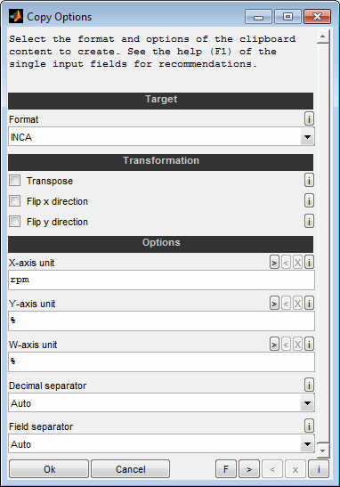
Format

Select the target format for the content to copy. Available formats are:
- Internal
  
  Use this format to exchange entire maps with axes between multiple instances or maps. Additionally the clipboard content can be used to interpolate a map to its axes. See “Load / replace template maps” for details.
- Spreadsheet
  
  Use this format to create clipboard content to paste into a spreadsheet software.
- INCA
  
  Similar format like ETAS INCA "Copy all data to clipboard" feature. It is not possible to insert a map with axes in INCA at once. The values and axes must be transferred one after the other by copying and pasting. Use “Copy map” to copy the map values in 2D or 3D view or use keyboard shortcuts to select and copy the map. To select and copy axes values you have to switch to 1D table view.
- MoTeC
  
  Use this format to create clipboard content to import in MoTeC software using “Import From Clipboard” feature. Remember to also enter the units and choose “Auto” for decimal and field separator or select the corrects values.
Transformation

Choose to transpose or flip the map before copying.
Units

For "MoTeC" format you need to enter the correct axes units.
Decimal separator

Choose the decimal separator for numbers to use when copying to clipboard. Use "Auto" for automatic detection depending on "Target".

MoTeC: .

Other: system default
Field separator

Choose the field separator to use when copying to clipboard. Use "Auto" for automatic detection depending on "Target".

4.5 Interpolate active map to new axes

The working page of the active map can be interpolated to the axes of a template map to load. The values of the map to load are irrelevant in this case - only the axes data will re regarded. If the dimension of the new template map differs from the dimension of the active map, also the reference page will be replaced to assure equal dimensions.

The procedure and options to load the new axes are similar to “Load / replace template maps”.

4.6 Invert active map

The working page of the active map can be inverted by tilting the map - one of its two axes is swapped for an axis corresponding to the w-values of the map.

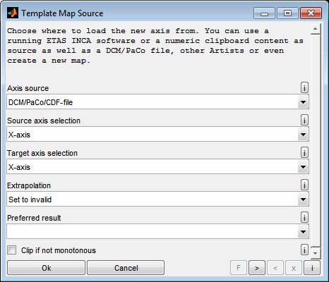
Axes source

DCM / PaCo / CDF - file

You can load the template map containing the axis from a DCM, PaCo or CDF file. The file will be asked and you can choose from all map labels in the file.
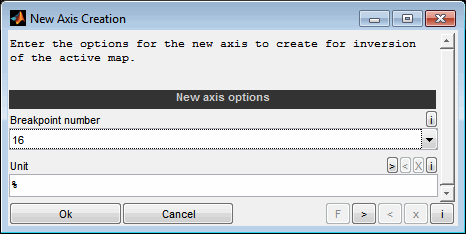
Create new

You can create a new axis without using any external source. When no template map was loaded the axis for map inversion is created by specifying its breakpoint number and unit.

INCA

A map can be retrieved from ETAS INCA software. Therefore INCA must be started and an experiment must be opened. The map will be retrieved from the active calibration page.
Clipboard

If you copied a map to clipboard this data can also be used to create a template. The clipboard data must be with axes. When no axes are loaded they are created as integer vectors starting at one. Sources for suitable clipboard content are spreadsheet software or calibration software like ETAS INCA (→ Copy all data to clipboard) or MoTeC (→ Export To Clipboard, CSV file).
Import from other Artists

You have the possibility to import maps from other currently opened MapArtists. The maps must be visible in 3D mode. A list of all available maps will be shown afterwards to select the ones to import. If you miss maps to import make sure they are shown in 3D mode in the other MapArtists.
Other maps

The axis can also be retrieved from other loaded maps directly.

Source axis selection

Decide which axis should be used from the "Axis source". The axis must correspond to the X-axis of the active map. For example, if you want to invert a map representing the torque over speed and load, the loaded axis must be a torque axis.

Target axis selection

Decide which axis of the active map should be replaced by the axis from the "Axis source". In this way, you determine the direction of the inversion. If the inversion is understood as tilting, you decide here the direction of tilting.

For example, if you want to invert a map representing torque (w) over speed (x) and load (y), you have two options.

If you want the result to be a map showing the load over speed and torque, select "Y-axis" as the target axis.
If you want the result to be a map that shows the speed by load and torque, select "X-axis" as the target axis.

Extrapolation

Decide how to handle points outside the axis areas. Default is to set the values to invalid (=NaN). You can also decide to keep the nearest value from the map or to extrapolate.

Preferred result

If the map is not monotonous, the inversion is not unambiguously possible, as there can be several solutions. In this case, you can decide whether you want to use the smaller or larger result.

Clip if not monotonous

This option is relevant for all points of the new axis that are above the map to be inverted.

Checked: For values to be inverted above the map the axis value corresponding to the maximum is determined.

Unchecked: The last axis value is determined for values to be inverted above the map.

5 Data points

Measurement data points are loaded to give the course of the map to create or to be displayed together with the map (Ctrl + o). This data may be scattered and must not be arranged to the map breakpoint values.

The data loading procedure is explained in the documentation of the SGE_Circus as it is common to all tools. We recommend that you read that section first as useful features like sample reduction, logical load conditions and calculated channels are explained there.

5.1 Load / append / replace data points

When loading data (Ctrl + o) you will be asked for files and channels to load. Normally you will choose three channels containing the x, y, and w values of the data points. You have to activate the “common axis” feature to ensure the equal number of x, y and w values. Calculated channels and the logical load condition can be used to load exactly the data you need.

The data points are organized in data points sets. Any number of data point sets can be loaded simultaneously. You can edit the color and description of the data points sets and switch their visibility (Ctrl + EnterData properties). Anyway even invisible data points take place for map optimization, smoothing and all other operations.

In addition to using the file load dialog, you can load sessions and data files by using drag and drop or the clipboard. To do this, one or more files can be dragged directly to a MapArtist session or inserted via keyboard shortcut (Ctrl + c / v). It is also possible to copy files directly to the clipboard as well as strings containing the file names line by line.

In case data points are already loaded the options for the data loading process like filename, sample rate and calculated channels will be proposed to easy replacing data. When multiple data point sets are loaded the first active one will define the options to propose. So when you need to get the settings of a specific data point set you can deactivate (Ctrl + Enter) all other to simplify the data loading process.

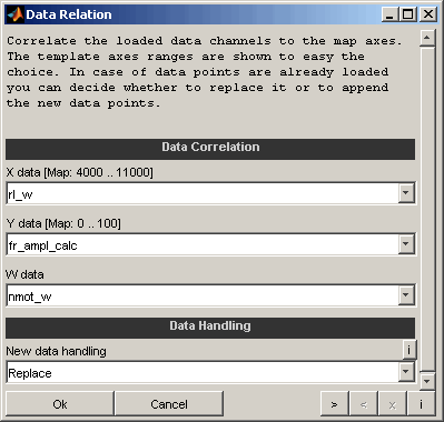
After loading the data and a template map you will be asked to the data correlation. Choose which channels loaded to use as x, y and w values. If you loaded a template map and do not want to create a new one the template axes ranges are shown to ease the choice.

In case data points are already loaded you will also be asked whether you want to replace them or to append the newly loaded data points. In case of adding data you will be asked to select a color for the new data point set. In case of replacing you have the option to only replace a single data point set instead of all.

If the loaded data contains NaN values these points will be removed automatically.

5.2 Interpolation mode

If you loaded a template map and do not want to create a new one you can alternatively load only two data channels. The third one is then interpolated from the active map. This feature is used to just display the operating area of the data file in the map.

5.3 Delete data

You can delete part of the loaded data points (Ctrl + d) that you don't need or want for map creation for example to remove spikes. You can either double click onto a data point or use the menu.

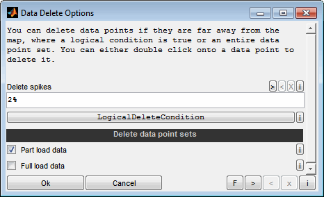
Delete spikes

You can delete data points if they are far away from the map. Define the distance threshold here either as absolute or percentage value. E.g. 2 or 2%. Leave this field empty if you don't want spike deletion.

Delete by logical condition

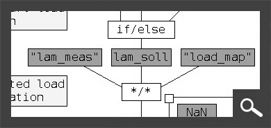
You can also delete data points where a logical condition is true. You can modify the condition in a graphical manner using the push button. Using the channel object you can access the following data:

"X" : X values (vector)
"Y" : Y values (vector)
"W" : W values (vector)
"I" : the map interpolated at the x/y values of the data points

The following picture gives an example for “Delete all points between xaxis 100 and 200”.

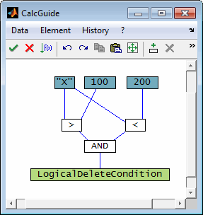
Leave the calculation empty if you don't want logical deletion.

Delete data point sets

It is possible to delete entire data point sets.

All conditions are combined with OR. So if at least one of them applies the point will be deleted.

Before deleting the data points a confirmation dialogue will be shown and the points noted for removal will be shown colored red. Rotation and zooming is enabled while the confirmation dialogue is present.

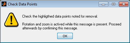
When a big number of data points will be deleted no red markup will be shown to avoid slowdown of the display.

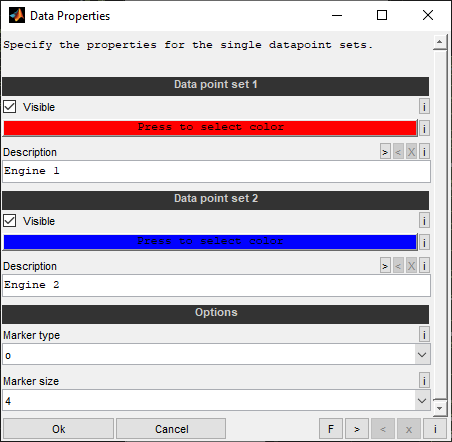
5.4 Data properties

When loading data points you can select to replace the existing data or to add to it. In the second case multiple data point sets will be created. Each set can have an individual color and description. Both can be modified (Ctrl + Enter). It is also possible to make single data point sets invisible. Anyway even invisible data points take place for map optimization, smoothing and all other operations.

The dialog additionally enables to edit the color of the marker points for each data points set separately and the marker type and size for all sets.

5.5 Check files

The files the data was loaded from is remembered and will be used e.g. to prefill the dialogs when reloading data. They can also be displayed using the data info ((Data) Info).

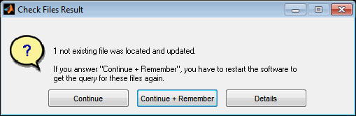
It may happen that files have been renamed or moved during the work or after reloading a session. Use the “Check files” option in this case to search the missing files and update their names and path automatically. Remember that sometimes it is not possible to find missing files. Especially all files must be located in the same directory. The option “Continue + Remember” allows you to save search results and apply them quickly next time without prompting. To reset these saved replacements, the software must be restarted or the corresponding option must be used when the message after automatic replacement is displayed.

5.6 (Data) Info

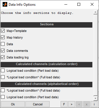
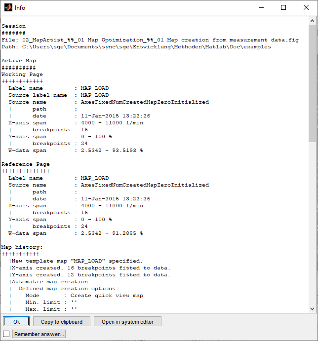
You can display some information about the loaded data and maps (Ctrl + Shift + i) like file names, comments, axes details, data loading / map history and calculated channels. This may be helpful to document the work done.

Calculated channels will be shown by opening them in the CalcGuide. This is just for display purpose. Modifications done in the CalcGuide will be discarded. In order to be able to find calculated channels quickly but also to be able to view the sequence of the calculation, they are displayed unsorted and sorted.

The data can be copied to the clipboard.

6 Mode, View

6.1 3D / 2D / table view

The MapArtist window has three main views – 3D, 2D and a table view. The 2D and 3D view can be shown simultaneously in a split mode. Switching between these modes can be done quickly using the keyboard shortcuts (Ctrl + 1, Ctrl + 2, Ctrl + 3, Ctrl + 5).

The view can be adjusted quickly by using mouse and keyboard shortcuts or the mouse – e.g. zoom (Ctrl + + / -, Mouse wheel) and rotate (Ctrl + Arrow, Ctrl / Shift + mouse wheel).

The axes labels and title can be modified. The axes labels are not always visible to maximize the view of the map if “Maximize axis area” is activated. Also the axes ranges can be modified and the axes ticks can be forced to accord with the map breakpoints (Ctrl + x). If “Axis auto” is checked in the menu the ranges will be chosen automatically.

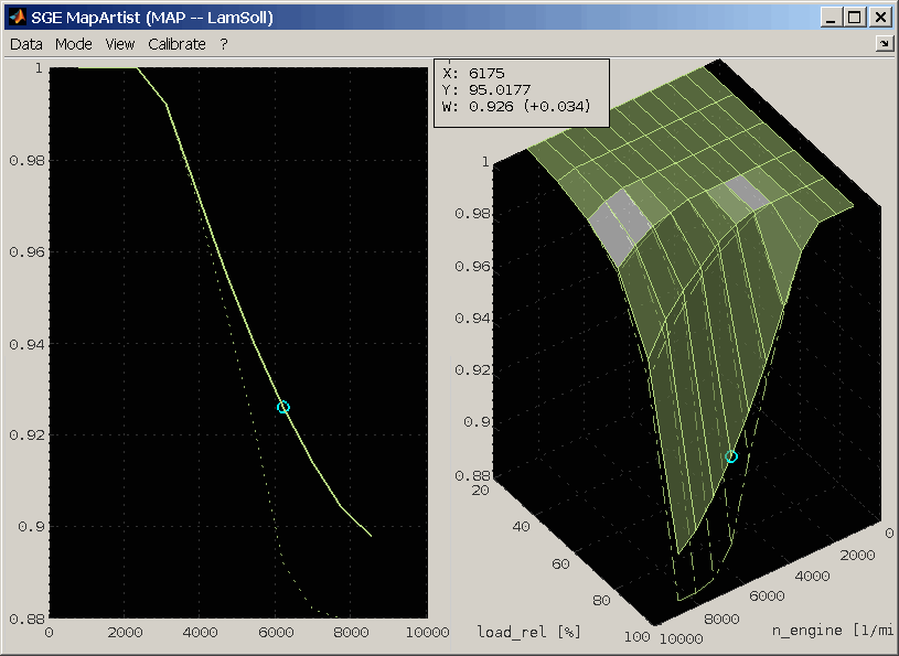
3D-Map / Iso-Diagram (Ctrl + 3, Ctrl + 5)

In 3D mode different display elements are available and can be individually activated.
Map (Ctrl + m)

The map color, transparency and light source are configurable. If you experience problems with the graphics display on some graphics hardware you could try avoid 0% transparency. Otherwise you will need to adjust the SGE Circus general graphics setting.
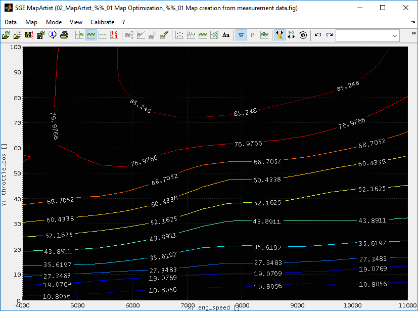
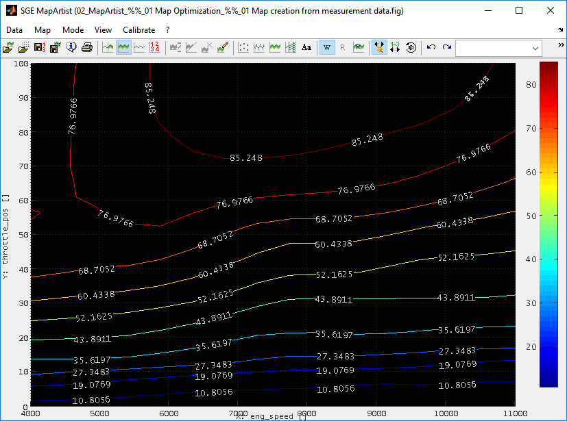
Contour plot

The number of lines or contour values and the display of values near the lines can be defined using the “Display options” menu item.
Data points (Ctrl + p)

The visibility of the data points can be activated separately above and below the map when you use the menu. The keyboard shortcut is used to switch both points simultaneously.
Error lines (Ctrl + l)

The error lines connect the data points to the map and ease the judgment of their deviation. Above the map they are colored white and under the map gray. The visibility of the lines can be activated separately above and below the map when you use the menu. The keyboard shortcut is used to switch both lines simultaneously.

Predefined standard views are available and can be toggled quickly using shortcuts (Ctrl + F12, Ctrl + r). It is also possible to adjust only the view without resetting the axes ranges (Shift + F12, Shift + r).

2D-Map (Ctrl + 2, Ctrl + 5)

Similar to the 3D mode the displayed elements are the map, data points and error lines. The view can be swapped between x and y axis (Ctrl + 2, Ctrl + 5).

The number of breakpoints to show in display direction upright to the screen can be configured (Shift + n). Only the active label defines the breakpoint values in this direction. All other labels are interpolated to the breakpoint values of the active label.

So for example when the 2D view is set to show the x axis, the y axis values to show are retrieved from the active label. The other labels are displayed interpolated to these y axis values while the x axis values remain individually for the single labels.

The lines are also colored white and gray. The data points are colored accordingly to the distance from the screen. This allows to judge their relevance for the actual breakpoint. The max. distance of data points to display can be selected using the corresponding menu item.
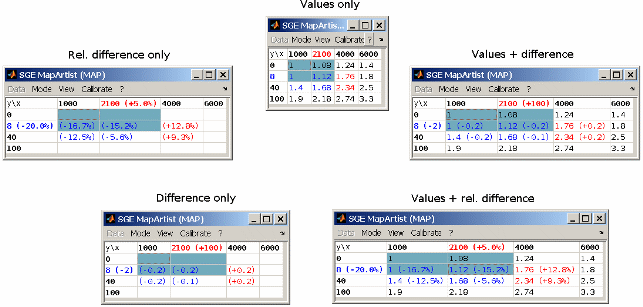
Table View (Ctrl + 1)

In table view different view modes are available. You can choose between different combinations of values, differences and relative differences (Ctrl + 1).

The differences between working and reference page are displayed in terms of color. Red indicates working page values bigger their reference page value and blue vice versa. The axes can be edited comfortably since monotony is only checked when the table view is exited. Remember that when the calibration rule is applied automatically, then axes monotony must be correct at any time. Turn off the automatic calibration rule application if you want to allow not monotonous axes temporarily.

The decimal places of the numbers to show can be modified. The setting is just for display purpose and has no influence to the data values itself.

The column width can be adjusted quickly to data changes using keyboard shortcuts (Ctrl + F12). Additionally a general setting can be used to define the extra space added to each column in terms of clear arrangement.

6.2 Working / reference page view

Depending on the selection in the menu either the working or reference page map is shown (F8). Additionally the reference map can be shown as a transparent background map with dotted lines while the working page is active (Ctrl + F8). Choose the grade of transparency and the color in the corresponding menu. By default the color is kept equal to the working page map color.

6.3 Data display reduction

To accelerate the display a sample reduction factor for the data points is used in 3D and 2D mode. 10 e.g. means that only every tenth data point is displayed. The option does not influence the created label. It is only used for displaying the data samples. "Automatic" means to automatically adjust the display reduction according to the performance of the computer.

“Automatic” is on by default. To use a specific data display reduction use the corresponding keyboard shortcuts (Ctrl + Shift + / - ). Once a specific reduction was chosen is remains active until automatic detection is reactivated (Ctrl + Shift + F12). It is also possible to enforce a specific reduction using the “Display options” menu item.

6.4 Display options

Using the “Display options” menu item enables to modify some display setting. It is possible to enforce a specific sample reduction as well as to configure the iso-contour plots.

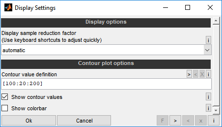
Display sample reduction factor

To accelerate the display a sample reduction factor for the data points is used in 3D and 2D mode. 10 e.g. means that only every tenth data point is displayed. The option does not influence the created label. It is only used for displaying the data samples. "Automatic" means to automatically adjust the display reduction according to the performance of the computer.

“Automatic” is on by default. To use a specific data display reduction use this option or the corresponding keyboard shortcuts (Ctrl + Shift + / - ). Once a specific reduction was chosen is remains active until automatic detection is reactivated (Ctrl + Shift + F12).
Contour value definition

The iso-contour plot can be customized. Enter a number here for the number of contour lines or a valid Matlab vector syntax for the values of the contour lines.

Examples:

20 : Create contour plot with 20 lines and automatic values.

[100:20:200]: Create a plot with lines from 100 to 200 in steps of 20.

[100:20:200 300:100:1000]: Create a plot with varying step size.

Many lines for the contour plot will slow down handling of the graphics. These definition is used for the data and error contour plot. This option does apply to the iso-contour plot as well as to the error iso-contour plot.
Show contour values

Activate this option if you want to display values next to the contour plot lines. This option does apply to the iso-contour plot as well as to the error iso-contour plot.

Show colorbar

Activate this option if you want to display a colorbar indicating the correlation of the map values and its color.

6.5 Background color

Using the corresponding menu item enables to adjust the background color of the 2D and 3D view.

6.6 Mark

Map values can be marked (selected) and will be highlighted then. This can be done using the mouse (Ctrl + Mouse button,Shift + Mouse button), keyboard and the menu function. Arbitrary map areas in 2D and 3D view can be marked/unmarked wiping the mouse while Ctrl key is pressed. The marker color, type and size can be modified using the corresponding menu items.

When points are marked several functions will ask to operate on the marked or all points when executed.

Using the menu function (Ctrl + m) enables you to use mark algorithms.

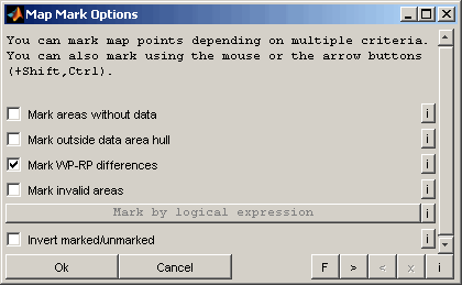
Mark areas without data

You can mark map points where no data points are nearby. This method may create "holes" in the map if there are no data points nearby the map breakpoints.
Mark outside data area hull

You can mark map points outside the data area. The data area is regarded as a convex hull around the data points. This method avoids to create holes in the map.
Mark WP-RP differences

You can mark map points that differ between reference and working page.
Mark invalid areas

You can mark map points that are invalid (NaN value).
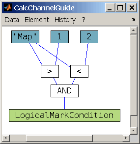
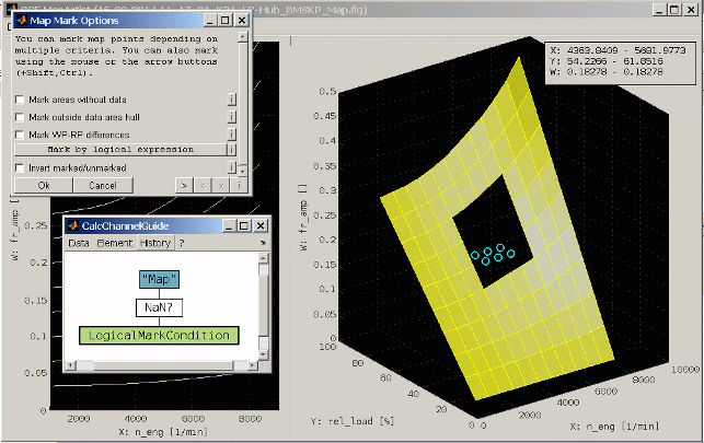
Mark by logical expression

You can mark map points where a logical condition is true. You can modify the calculation in a graphical manner using the push button. Using the channel object you can access the following data:

"Map" : map-matrix-values (x-axis is column index, y-axis is row index)
"AxisX" : x-axis-vector (row vector)
"AxisY" : y-axis-vector (column vector)

The following picture gives an example for “Mark all points with map values between 1 and 2”.

Invert marked/unmarked

You can finally invert marked / unmarked points. The inverting is done after all other mark actions.

The different mark methods are combined with OR.

6.7 Cursor

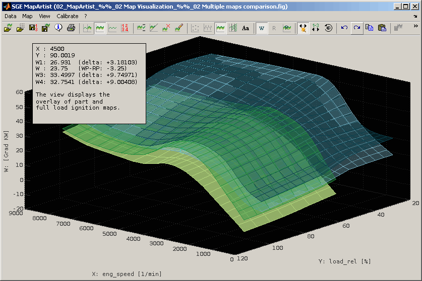
When map points are marked a cursor view is activated in the top left corner. The position of the cursor view can be modified by dragging it with the mouse.

It displays the values of the current point or current range if multiple points are selected. Also the difference working to reference page and absolute / relative error referenced to data points is shown.

In case multiple labels are loaded their difference to the active label is shown.

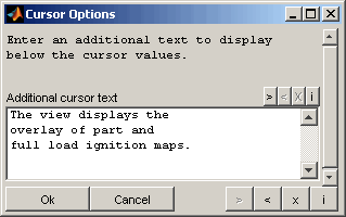
The cursor can also display an individual text below the data values. Use the corresponding menu item or double click the cursor to edit the individual text. Remember that the cursor and therefore the individual text will only be displayed when map points are marked.

7 Map creation and optimization

The main target of the MapArtist is to create a plausible map that matches the data points. Therefore a set of functionality is available to create and smooth the map and axes distribution.

When points are marked you will be asked whether the operations should be done for all or only the marked map points.

7.1 Map calculation

The map calculation (Shift + c) generates the map values to fit the data points using multiple algorithms. Thus the map calculation can only be performed when data points are loaded.

Workmode

Display template map and data points

The data and the map will only be displayed and not changed e.g. to judge the error or create an iso-contour plot.
Create quick view map

This mode is very quick. But without the optimization the map is more a quick guess than a good fitting map.
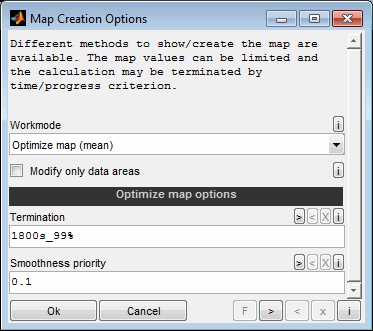
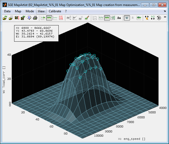
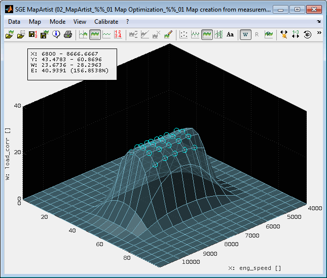
Optimize map

With optimization the map is fitted as good as possible to the data. Special methods to treat areas without data are used. The optimization progress is shown graphically and can be interrupted at any time. In this case you can choose to use or discard the intermediate result. The direction of optimization can be chosen between mean, which means that the map fits the data points best and direction above or under, which means, that the map will be optimized to hull the data points.
Gaussian Process Model

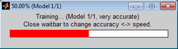
The map is created by optimizing a Gaussian Process Model to fit the data' points. A Gaussian process model is a statistical model, where a set of variables associate the axes values with a stochastic distribution of the map value. In general this is suitable to fit arbitrary map shapes with reduced risk of overfitting. As the optimization is very resource extensive the calculation may last very long or even be impossible. During optimization a progress bar is shown. By closing it you can abort the optimization prematurely or change a trade off level between accuracy and speed. In general you should prefer accuracy.

Fit plane

A plane is fitted to the data. The order can be chosen. If points are marked in the map only the marked points will be calculated or optimized.

Modify only data areas

You can choose if you want to calculate the whole map or only ares where data points exist. The data area is regarded as a convex hull around the data points.

Termination

This option is only valid for the "Optimize map" modes and must be empty for all other modes.

During smoothing a progress bar is shown to judge the progress. The progress shown corresponds to the remaining deviation from the map to the data points. In practice the deviation will not be reduced to zero because the map will not be able to fit the data points perfectly as the breakpoint number is limited and data points are influenced by measurement tolerances. So the waitbar will stabilize at any value but not reach 100%.

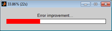
You can limit the time and/or the progress for the optimization in the options dialog. Define as string ending with ''s'' for seconds or/and ''%'' for a relative percentage limit. E.g.: 10s 80% 10s_80%

The map view will be updated regularly during optimization to judge the progress. When the result is satisfying the entire optimization process can be terminated by closing the waitbar window.

Smoothness priority

This option is only valid for the "Optimize map" modes and must be empty for all other modes.

It specifies the priority to consider for the smoothness of the map during optimization. 0 means to fit the map to the data points as good as possible without regarding its smoothness. Higher values increase the smoothness of the map at cost of its accuracy to fit the data points. A value of 1 means approximately the same priority of smoothness and accuracy. In general the value should be as small as possible. Values of about 0.1 may be a suitable starting point.

There is no need to enforce the desired smoothness of the map by using high values for this option because separate map smoothing algorithms are available. See the following section.

7.2 Map smoothing

After calculating a map it is generally a good practice to process some smoothing (Shift + s). Mostly it is possible to get more plausible maps without increasing the deviation to the data points too much. When points are marked you will be asked whether the operations should be done for all or only the marked map points.

Generally spoken the best smoothing settings must be evaluated for every use case.

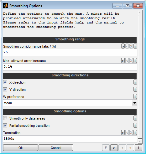
Smoothing corridor range

Around the map a "corridor" will be created with the width of the chosen range. Then the smoothest possible map inside this corridor is created. This methods always tries to straighten the map and may change the course of the map. It is recommended to apply a "Max. allowed error increase" if data points are loaded.

The corridor range entered here can be relative or absolute. If the value ends with % it is regarded as relative in percent of the map value. This may lead to unwanted behavior if the map values are close to 0. Use together with the "Max. allowed error increase" option.

Corridor smoothing only tries to smooth the map in the directions that are activated.

Max. allowed error increase

You can limit the error increase due to smoothing to a certain value. This is a very powerful option to retrieve smooth maps without changing the main map course. This option enables to use big or even unlimited “Smoothing corridor ranges”.

The value entered here can be relative or absolute. If the value ends with % it is regarded as relative in percent separately for each map point. This may lead to unwanted behavior if the map values are close to 0. E.g. 1% means that every map point can be modified by the algorithm to get a smoother map until the mean absolute error increases by 1% of the map value. Without % it is regarded as an absolute value in units of the map.

The values entered here do not have a quantitative meaning. Due to calculation strategies 1% error increase will not exactly be 1% of the map value. The right value to use must be evaluated for every use case.

Generally it is recommended that areas outside the data are adjusted roughly before smoothing with error limit. This can be done by marking only this area and smoothing without error limit first.

X / Y direction

The axis directions to smooth in can be chosen. If you experience unsatisfying smoothing results you may try to smooth only one direction or both directions sequentially.

W preference

The vertical W preference of smoothing can be chosen between "mean", which means that the map fits the data points best and direction "above" or "under", which means, that the map will be smoothed to hull the data points. This option will only have an effect if data points are loaded.
Smooth only data areas

You can choose if you want to smooth the whole map or only ares where data points exist. The data area is regarded as a convex hull around the data points.
Partial smoothing transition

Activate this option if a even connection to the neighboring areas should be created for partial smoothing. If this option is deactivated, the area to will be smoothed without taking into account the transition to the other areas. This option is only relevant if parts of the map were selected before smoothing or if the area to be smoothed was reduced by the “Smooth only data areas” option.

The following two figures show the influence of this option. With active option (left) the smoothed area has an even transition to the neighbouring areas. Without the option (right), this transition is not taken into account and is therefore not smooth.
Termination

During smoothing a progress bar is shown. Because the smoothing process is split into different phases with different proceeding you will recognize that the progress shown is not linear. The waitbar will speed up and slow down alternately. When it stops for too long you have the possibility to skip to the next phase by closing the waitbar window and choosing the corresponding option in the dialogue shown afterwards.

You can limit the time and/or the progress for the smoothing in the options dialog. Define as string ending with ''s'' for seconds or/and ''%'' for a relative percentage limit. E.g.: 10s 80% 10s_80%

The map view will be updated during smoothing to judge the progress. When the result is satisfying the entire smoothing process can be terminated by closing the waitbar window.

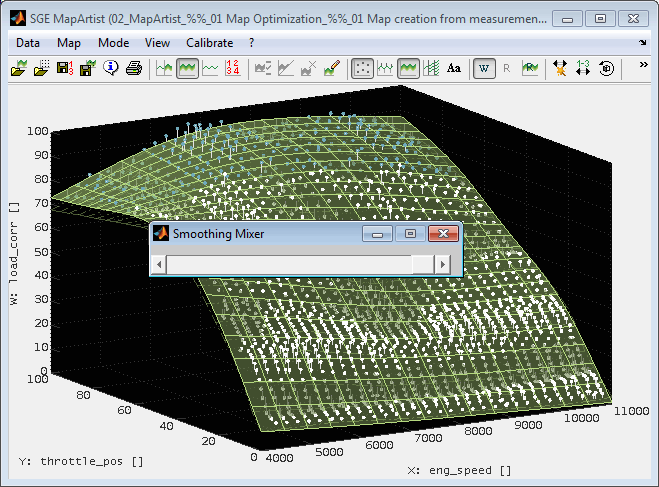
After termination of the smoothing the map points that were restricted to smooth by the corridor width or the error criterion will be marked to be able to judge the smoothing options chosen. These marks will be removed when resetting the view, recalling the function or using the following mixer.

Smoothing mixer

A mixer will be shown after finishing the automatic smoothing to balance the smoothing result between the initial map before smoothing and the map resulting from the automatic smoothing process.

7.3 Axes optimization

The axes optimization is used to modify the axes breakpoints in a way that the map fits the data points in an optimal way (Shift + a). Thus the map calculation can only be performed when data points are loaded.

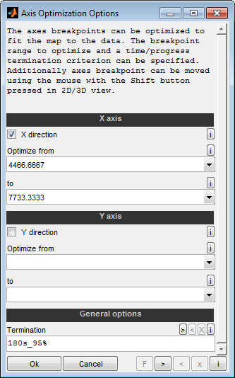
The axes optimization can be restricted to single directions and breakpoint ranges. You can limit the time for the axis optimization. Define as string ending with ''s''. E.g.: 10s.

When points are marked the axes optimization will only regards these points. Therefore it is possible to optimize axes with focus on specific map regions.

In general axis optimization is only reasonable if the data values are equally distributed. If the data was measured with discrete values only the axis optimization will fit the axes breakpoints to these data values.

After axes optimization the map calculation should be repeated to again fit the map values to the data points.

8 Calibration

After creating a base map using the map optimization and smoothing features or loading a existing map you probably want to fine tune it manually or tool assisted using your experience and regarding the constraints given by the purpose of the map.

The MapArtist provides a set of features to do this

8.1 Standard operations

To modify the map one or multiple points must be marked. All operations refer to the marked points only.

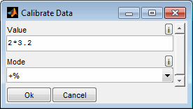
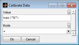
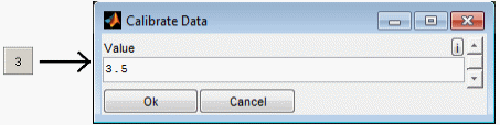
Value

Enter a numeric value or "n(an)" or a calculation. Values can be specified either directly or as a simple calculation rule. In the calculation rule, the placeholders "X", "Y", and "W" can be used to access the current values of the map or the axes. Additionally "XMAX", "XMIN", "YMAX", "YMIN", "WMAX" and "WMIN" can be used to access the extrema.

Examples:

100 : Numeric value

nan : Invalid value

2*pi/360 : Calculation rule

sin(2*pi) : Calculation rule

tan("W") : Calculation rule including map values

tan("W")*"X"^2 : Calculation rule including map and x-axis values

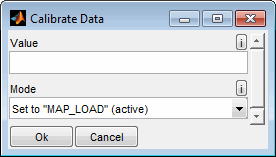
Mode

The standard operation are:

= : Set to value (numeric or n[an]).
+ : Add value (also negative to subtract).
* : Multiply with value.
/ : Divide by value.
+% : Add relative value in percent.
SetToReferencePage: Set to value of reference page of active map.
SetInvalid : Set to invalid (NaN).
Set to "label" : Set to value of another map. Interpolation will be done in case both maps have have different axes. Outside the axes range the interpolation will clip the last map value.
Increment / Decrement

Most of them are accessible via keyboard shortcuts and you can also increment/decrement using the mouse wheel. See the keyboard shortcut section for details.

Especially using the keys for the digits and – allows to directly input a new value for the marked map points.

When the error lines (and therefore the error calculation) are turned on and only one point is marked and modified, the color of the mark indicated the error trend. When it is green, the error was decreasing by the modification. When it is red, the error was increasing.

The axis values are modified you will be asked whether to adjust the map accordingly by interpolation or extrapolation. The decision can be remembered. In this case you will not be asked again until the software is restarted.

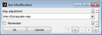
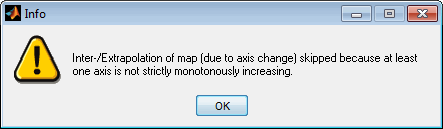
Interpolation / extrapolation can only be performed when the axes are strictly monotonously increasing. You will be informed when this condition is not met.

8.1.1 Invalid map points

If you set points to invalid, they are filled with NaN (not a number) and made invisible. This creates holes in the map. Sometimes this is e.g. useful to not show border areas where no data points exist. You can not mark invalid points directly any more. To mark them you must mark areas around to include them or use a logical mark condition.

To use a map in the ECU or to save it to calibration parameter file you must fill all invalid point with numerical values.

8.2 Advanced operations

8.2.1 Interpolate

You can do a linear interpolation of marked sections of the map in x or y direction (Shift + x / y). The border values of the section is kept and the intermediate values are interpolated.

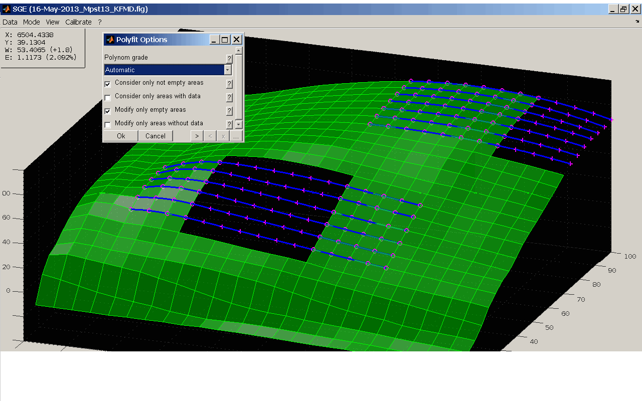
8.2.2 Polynomial / exponential fit

Similar to the extrapolation you can to a interpolation. Similar options are available.

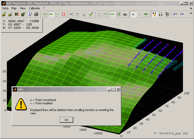
When doing polynomial, exponential fits or extrapolations the fitted curves are displayed as lines as well as the considered and modified points. To remove them you can recall the interpolation functions or reset the view.

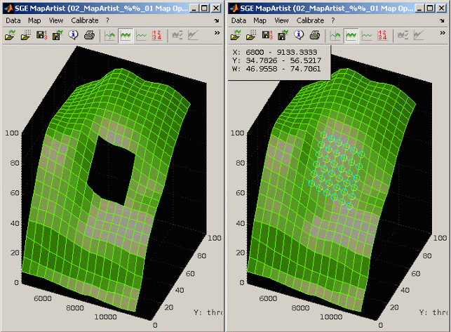
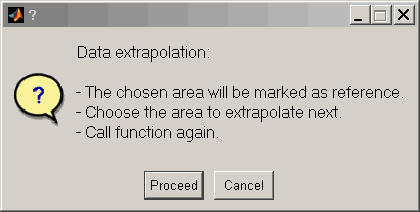
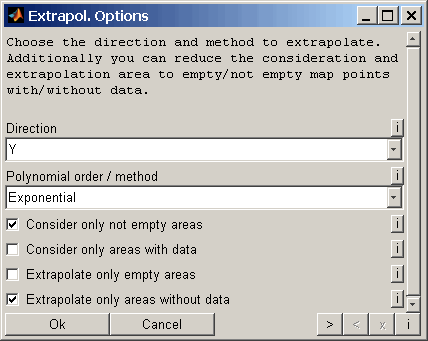
8.2.3 Extrapolate

You can do an extrapolation of sections of the map (Ctrl + Shift + e). This is done using a two step procedure. First you mark a reference area and call the extrapolation function. Then you mark the area to extrapolate and call the function again.

The two areas must overlap in only one direction. Some options are asked:

Direction

Choose the direction to extrapolate in.
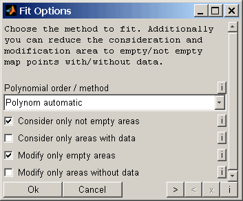
Polynomial order / method

In the reference area the map points are fitted by a polynomial or exponential curve in the chosen direction. The curve is then used to calculate the values in the extrapolation area. Choose the polynomial order or exponential method here. The maximum value depends on the size of marked area.
Consideration areas

You can reduce the map points to consider for the curve fit to the not empty (NaN) points or / and to the map points with data points nearby. This is useful as you can mark big areas but use only part of it for extrapolation. So you can easily extrapolate scraggy map bounds because you can mark a rectangular area but only consider the not empty part as reference.
Extrapolation areas

Similar to the consideration area you can also reduce the extrapolation area.

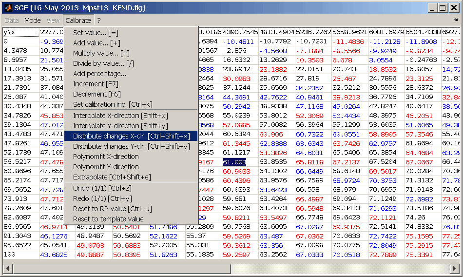
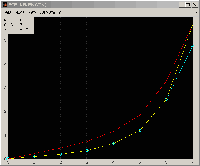
8.2.4 Distribute changes

Sometimes only parts of the map are modified and the changes should do a smooth transition to the neighborhood areas. Imagine you correct the full load breakpoint only but want the change transferred to the part load area with decreasing influence.

Use the “Distribute changes” (Ctrl + Shift + x / y) function to achieve this. You need to mark the transition areas as well as the border of the changed are. The difference between the reference and working page at this border is then linearly distributed.

In the following figure the cyan line is the reference page. The yellow one is the modified map - only one breakpoint is changed. After distributing the change the red line is created.

8.2.5 Limit gradient

If the map should agree with limitations regarding its gradient these restriction could be applied automatically (Ctrl + g). For example it could be necessary that a map is strictly monotonously increasing in x direction.

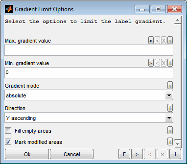
The following options are asked:

Max. gradient value

Enter a scalar numeric value to use as the maximum gradient limit. Value may be positive as well as negative or zero. Leave empty to not restrict the max. gradient and set to "Min. gradient value" to force a fixed gradient.
Min. gradient value

Enter a scalar numeric value to use as the minimum gradient limit. Value may be positive as well as negative or zero. Leave empty to not restrict the min. gradient and set to "Max. gradient value" to force a fixed gradient.
Gradient mode

The limit value entered above may be absolute or gradient.

Absolute:The delta between neighbor label values will be limited directly.

Gradient:The gradient between neighbor label values will be limited. Therefore the axes breakpoint distance is considered to calculate the gradient.

Examples for limit value 2:

absolute: label [1 1 10 20] -> [1 1 3 5]

gradient: axis [0 10 20 40] [0 10 20 40]
Direction

Choose the direction to operate. If label points are marked, only the marked points are regarded.
Fill empty areas

If selected empty areas will be filled. Otherwise empty areas will be skipped.
Mark modified areas

If selected the label areas modified due to gradient limiting will be marked.

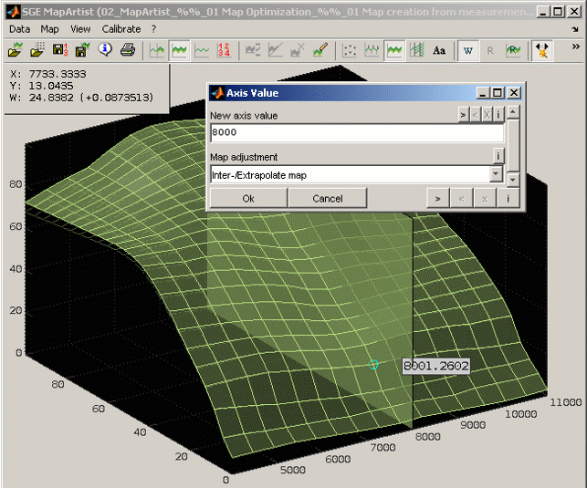
8.2.6 Graphical axes modification

In addition to the automatic axis optimization in 3D view and the manual edit of axis points in table view you can directly drag axis breakpoints in 2D/3D view with the mouse while pressing the shift key (Shift + Mouse button).

Proceeding:

Make sure to have exactly one map point marked.
Press the Shift button, click to the marked point and keep the mouse button pressed.
Move the mouse once far away to the screen border to unsnap the axis point.
Place the axis point as desired and release the mouse button. The axis pane and value are shown during modification.

After releasing the mouse you will be asked to confirm the new value and if you want to interpolate / extrapolate the map to the new axis value.

8.3 Copy / paste

You can copy and paste parts of the map or the whole map using the clipboard (Ctrl + c / v, Shift + w). The format is suitable to paste into a spreadsheet software. Additionally entire maps with axes can be copied to clipboard using different target formats. See “Fehler: Referenz nicht gefunden” for details.

Additionally you can load sessions and template data files by pasting them into a MapArtist session. Before you have to copy them directly to the clipboard or as strings containing the file names line by line.

Using copy and paste in table view will always handle the map/axes values – even if the display mode is set to show e.g. differences.

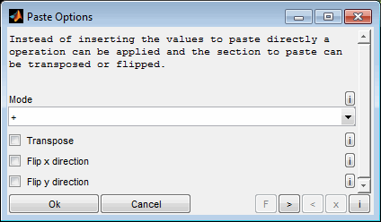
Using the extended paste mode (Ctrl + Shift + v) enables you to apply operations like addition, subtraction, multiplication, division or max/min selection when pasting the values. This can be used e.g. to add two maps. It is also possible to transpose or flip the data before pasting.

The decimal separator used for copy / paste actions can be set in the SGE Circus preferences – by default the operating system setting is used.

8.4 Set to reference page value

You can set parts of the map or the whole map to the value(s) of the reference map (Ctrl + u).

8.5 Conversion rule

Usually a label is implemented in a ECU using computer data types and then calculated to physical values using a conversion formula. This may lead to a restriction of the value range and force a incrementation. To consider this while editing a label the conversion rules for the label and axes may be specified (Ctrl + k).

Initially the values are set to the A2L values if available, e.g. if the label was retrieved from ETAS INCA software. The values are also remembered in relation to the label name in a database. They will be retrieved from database again if you import a map from calibration parameter file or create a new label. Therefore it is important to enter the exact label name when creating a new label.

You man enter values differing from the ECU conversion to ease manual map editing. But best practice is to keep the ECU conversion and use the manual editing increment gain setting to adjust to a suitable for manual incrementation and decremention.

The conversion rule may be applied by manual invocation (Shift + k). When the corresponding option is enabled it will be applied automatically whenever the map is manipulated, e.g. after automatic map creation, smoothing, pasting and so on. When automatic application of the conversion is disabled the increments are just used for manual incrementation. All other map manipulations do not consider the conversion rule then.

For manual map editing (incrementing, decrementing) in general the increment from the conversion rule is used. To adjust to the practical needs a gain factor can be set. The gain factor does not influence the conversion rule. It is just used for manual map editing.

Besides the settings here the A2L conversion rules may be considered when saving the map to calibration parameter file or ETAS INCA software.

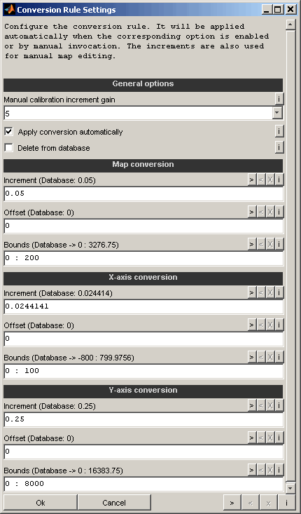
Manual calibration increment gain

For manual map editing (incrementing, decrementing) in general the increment from the conversion rule is used. To adjust to the practical needs a gain factor can be set. The gain factor does not influence the conversion rule. It is just used for manual map editing.
Apply conversion automatically

When enabled the conversion rule is applied automatically whenever the map is manipulated, e.g. after automatic map creation, smoothing, pasting and so on. If not enabled the conversion rule is only applied when invoked manually using the corresponding menu option (Shift + k). Besides the settings here the A2L conversion rules may be considered when saving the map to calibration parameter file or ETAS INCA software.
Delete from database

If enabled the info for the actual label will be removed from database. This option may be used to remove incorrect or outdated data from database. If the database contains multiple entries for a label name only one will be deleted.
Increment / Offset

The values will be forced to agree with the offset and increment if the conversion rule is applied. The increment does also influence the step used while editing the map manually.
Bounds

The values will be limited to the range entered if the conversion rule is applied. Specify scalar values separated by colon or spaces, e.g. 0 : 100 for a range from 0 to 100. Use inf/-inf for unlimited ranges, e.g. -inf : 100. Leave empty to not apply bounds.

9 Save session

The whole session including data can be stored as file (Ctrl + Shift + s). After re-opening the whole functionality can be used again immediately.

Session files can be opened the same way as data files or using the SGE Viewer. Session files may get very large as they contain the loaded data.

Apart from saving a session it is possible to save maps to files and transfer datasets to ETAS INCA software, see section “Save maps“ for details.

10 Present, print, organize

10.1 Copy view to clipboard, print

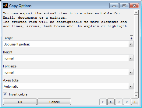
To be able to use the maps and data also for presentation purposes, the MapArtist makes it available to export the actual view into the clipboard or file formatted in a way that is suitable to be useful for different targets (Ctrl + Shift + c).

Document
Email
File
Printer

This can be different sizes of clipboard content. "Email" and "Document" are specially sized to fit into a email or document software. Some paper formats are also available and all windows can be printed and saved to various file formats.

The created window is configurable. So you can move elements like legend or cursor boxes. It is also possible to add lines, arrows, text boxes etc. to the window to explain or highlight.

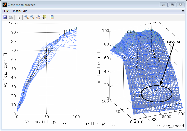
During creation some options will be asked to define the base layout of the window.

After closing the window the content will be copied to clipboard and can be pasted / used in the target software.

10.2 Window handling

Since the SGE Circus offers to open a considerable number of windows an automatic window handling feature is implemented. Using the corresponding menu item enables to arrange all or a subset of the windows of the current session.

Close windows

This feature enables to close visible and invisible windows automatically.

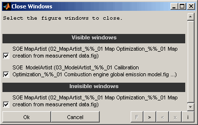
Windows

Select which windows to close. The windows will be closed without saving anything and without any further confirmation. Visible and invisible windows will be listed separately.

Resize windows

This feature enables to automatically set windows to fixed sizes or to maximize, minimize and restore them.

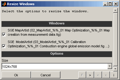
Windows

Select which windows to resize.
Size

Select the desired window size. It is possible to maximize, minimize and restore windows. Additionally a set of fixed standard sizes are available.

Arrange windows

This feature enables to automatically arrange windows.

Window arrangement

Select the layout of the arrangement. It is possible to maximize, minimize, restore or close all selected windows. Additionally column and row based layouts are available.

Example: "2-3 of 5 rows" means that the screen is split into 5 rows and the second and third row is used for the layout.
Target monitor

Select the target monitor for the windows to arrange in case of multiple monitors are connected to the computer.
Windows

Select which windows to include into the arrangement.

Toggle windows periodically

This feature enables to automatically toggle windows to create kind of a movie. This can be used to compare windows.

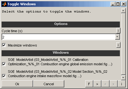
Cycle time

Select the the time to wait before activating the next window.
Maximize windows

If enabled the windows will be maximized before toggle to ensure identical size.
Windows

Select which windows to toggle periodically.

11 General information

Duplication, processing, distribution or any form of commercialization of the documents content beyond the scope of the copyright law shall require the prior written consent of the SGE Ingenieur GmbH. All trade and product names given in this document may also be legally protected even without special labeling (e.g. as a trademark).

MATLAB, Simulink and Stateflow are registered trademarks of The MathWorks Inc., Natick, MA, USA.
INCA is a registered trademark of ETAS GmbH, Stuttgart.
Microsoft, Windows and Excel are either registered trademarks or trademarks of Microsoft Corporation in the United States and/or other countries.
Apache and OpenOffice are trademarks of The Apache Software Foundation.

The SGE Circus includes Third Party Software. For details please refer to the → SGE Circus documentation.

SGE Ingenieur GmbH – www.sge-ing.de

Contents