SGE ModelArtist – User Manual
www.sge-ing.de – Version 1.62.67 (2022-07-24 22:21)
1 Introduction
The SGE ModelArtist is a tool to visualize and model multirelational data as well as to enable model based calibration.
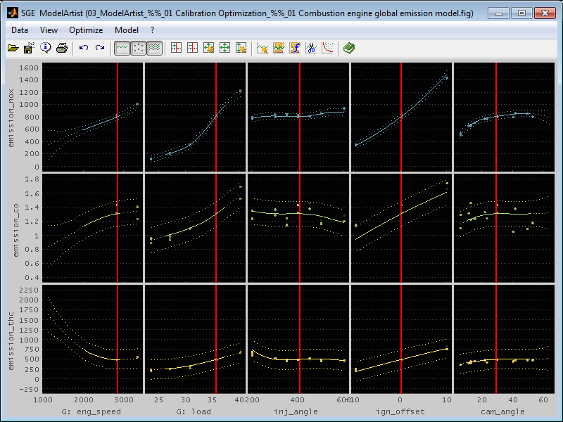
You can load an arbitrary number of input and output channels and the correlation between each input / output combination is displayed in a matrix intersection view. Cursors and zoom functionality is used to adjust the display to the relevant data.
Different kinds of models can be trained to fit the data and enable the homogeneous display of scattered data as intersection plots. Thus the optimization of the calibration of systems with multiple inputs is assisted.
This manual contains information concerning specifically the SGE ModelArtist only. The SGE ModelArtist is part of the SGE Circus. For help topics regarding general features please refer to the corresponding documentation accessible using the links below.
1.1 SGE Circus user manualThe SGE Circus documentation makes available general information regarding data loading procedure, input handling, preferences, history and other topics concerning all tools. |
1.2 SGE CalcGuide user manualThe SGE CalcGuide is a tool to implement calculation routines by creating graphical flow chart diagrams - included with all tools. |
|
|
|
1.3 SGE Circus videos (external) |
|
|
|
For information regarding the version dependent software changes please refer to the Release notes accessible using the corresponding menu item inside the SGE Circus.
2 Keyboard shortcuts, mouse gestures
Many functions are quickly accessible via keyboard shortcuts. For a list of available keyboard shortcuts, see the list below. In addition, the entries in the menus and context menus as well as the tooltips of the toolbar point to shortcuts.
|
Data Handling |
|
|
Load data... |
|
|
Save data... |
|
|
Paste files from clipboard into present session... |
|
|
Data info... |
|
|
Save session... |
|
|
Rename inputs / outputs... |
|
|
Copy cursor values to clipboard |
|
|
View |
|
|
Zoom in x / y direction |
|
|
Mouse right button drag |
Pan in x / y direction |
|
Increase / decrease / automatic display reduction |
|
|
Increase / decrease max. data distance... |
|
|
Reset ranges of all axes in x- and y-direction. Activate automatic display reduction. |
|
|
Fit all y-axes |
|
|
Reset range of actual x- and y-axis |
|
|
Set x-axis range... |
|
|
Set y-axis range... |
|
|
Double click cursor line |
Set cursor position... |
|
Toggle visibility of inputs |
|
|
Toggle visibility of outputs |
|
|
Toggle visibility of data points |
|
|
Toggle visibility of model |
|
|
Ctrl + f |
Toggle visibility of 95% confidence interval |
|
Color data points / model... |
|
|
Model |
|
|
Train model(s)... |
|
|
Delete model(s)... |
|
|
Export model(s)... |
|
|
Model section... |
|
|
Optimization |
|
|
Shift + o |
Optimize calibration parameter... |
|
Optimize calibration system... |
|
|
Miscellaneous |
|
|
Show manual... |
|
|
Show keyboard shortcut manual... |
|
|
Undo (views, models) |
|
|
Redo (views, models) |
|
|
Copy window to clipboard..., Print window... |
|
|
System optimization (waitbar shortcuts) |
|
|
Show status... |
|
|
Show system signals... |
|
|
Show progress course... |
|
|
Ctrl + s |
Save calibration parameter file... |
3 Features
The main features of the SGE ModelArtist are listed in this introduction. For details please see the following sections.
Visualization
Data formats MDF3/4, ASCII, Diadem, FAMOS, Horiba-VTS, IFile, Kistler *.ifi, BLF/ASC CAN files, Excel*, OpenOffice*, MATLAB, Magneti Marelli, MoTeC, 2D, Get, Tellert, Keihin (* if Apache OpenOffice or Microsoft Excel is installed)
Data import from MATLAB workspace, function calls, Simulink simulations and DLL output
Definition of any calculated channels including features like map interpolation and Simulink systems integration. By direct use of filters and calculations, the preprocessing of data can often be eliminated.
Automatic down-sampling for flowing display even of large amounts of data
Data points, model and confidence display
Zoom, cursors
Scatter plots based on training/test and model data
Data correlation plots to quickly judge the inputs relevance
Model sections to reduce model dimensions for visualization
Modeling
Gaussian, QuickView, Linear, Polynomial, Exponential models
Adjustable split of data into training and test data
Data clustering to reduce tolerances and speed up model training
Training options, accuracy configurable
Correlation plots, error plots, outlier removal
Input interaction plots
Pareto plots
Model export / import
Calibration Parameter Optimization
Automatic optimization of calibration parameters (maps, curves)
For example emission optimization, closed loop controller calibration, cam timing optimization
Calibration parameter source from DCM/PaCo/CDF file or INCA (*)
Tolerance criterion to enable generation of smooth maps
Integration of already existing partial calibration
Free definition of the optimization target as taking into account limits, operating point weighting

Calibration System Optimization
Automatic calibration of entire ECU functions for mapping a measured model behavior
For example exhaust gas temperature model, torque model, load detection
Algorithms to achieve smooth plausible results
Integration of already existing partial calibration
Free definition of the optimization target as taking into account limits, operating point weighting
Graphic Export
Configurable export of the actual screen to the clipboard
Ready formatted for email or office software. Reports made easy.
Axes, fonts, sizes adjustable. Adding notes, highlights, etc.
4 Data
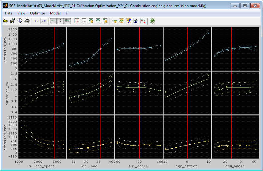
Data points are loaded for display purposes, to train models or to perform optimization. The data may e.g. result from measurements or simulations. You can load any number of input and output channels. Input channels will be displayed as horizontal axes and output channels as vertical axes. This way the intersection plots are generated.
In a simple example a testbench measurement is loaded and engine speed and throttle position are selected as input channels and load and torque as output channels. In a more realistic use you will for example also select lambda, ignition timing and cam timings as inputs and emission concentrations, cylinder mean pressures, centers of combustion and specific fuel consumption as outputs.
The data loading procedure is explained in the documentation of the SGE_Circus as it is something all tools have in common. We recommend that you read that section first as useful features like sample reduction, logical load conditions and calculated channels are explained there.
4.1 Data preprocessing
The quality of the data loaded is essential for the model quality as well as for the model training effort in terms of memory usage and computing time. To ensure optimal results it is recommended to check the data before loading for measurement inaccuracies and drifts. At least use the correlation and errors plots after model training to check the results.
If the model training duration or memory effort exceeds a reasonable limit you should first try to reduce the number of data points by data preprocessing – for example points with similar input value combinations should be reduced to single points by calculating the average values of input and output value. This can also happen automatically during the model training by using the clustering feature – see “Train model“ for details.
4.2 Load data
You can load data points initially after starting the ModelArtist. It is also possible to reload data (Ctrl + o) afterwards. Choose all input and output channels to display at a time. You have to activate the “common axis” feature to ensure the equal number values for each channel. The logical load condition can be used to load exactly the data you need and calculated channels assist you to create channels with new features or combinations of multiple channels.
After loading the data a dialog will be shown to select the output channels from the list of all channels loaded.
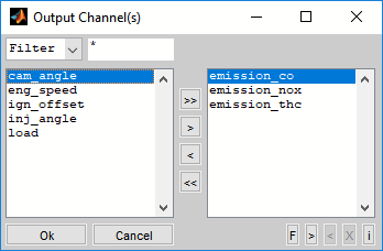
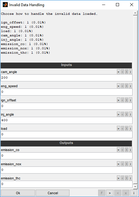
If the loaded data contains invalid values (e.g. NaN, inf), you must decide how to handle them. No invalid values are allowed in inputs. They are allowed in outputs, but may be undesirable. You can therefore decide for each input and output whether invalid values should be replaced with a fixed value or whether invalid values should be removed.
Inputs
You have the following options for handling invalid data in input channels:
Enter a scalar numeric replacements value.
Leave empty (default) to remove this data point for all inputs and outputs.
Examples:
0→ replace all invalid data with 0 values.
→ remove all invalid data.
Outputs
You have the following options for handling invalid data in output channels:
Enter a scalar numeric replacements value.
Enter "NaN" to replace with NaN values.
Leave empty (default) to remove this data point for all inputs and outputs.
Examples:
0→ replace all invalid data with 0 values.
NaN→ replace all invalid data with NaN.
→ remove all invalid data.
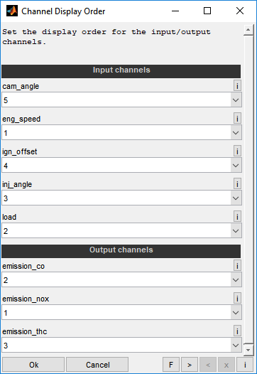
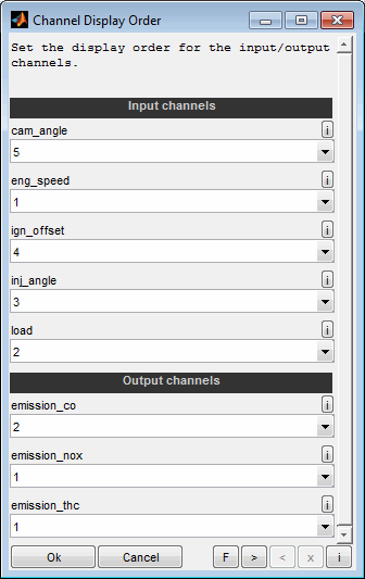
Afterwards a dialog shown allows to modify the display order of the loaded input and output channels. The order just influences the display and does not effect the model or optimization. By selecting the same order number for multiple outputs they will share the same axis. In contrast the order numbers of the inputs must be unique.
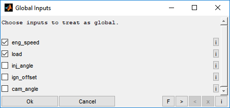
Finally the input channels to define as global will be asked. Global channels define e.g. the operating point and will not be judged as a variable value to optimize the outputs. Optimization will be done separately for different global input value. For example engine speed and engine load/torque usually are global inputs.
If the loaded input data contains NaN or infinite values these points will be removed automatically for all channels. If the loaded output data contains NaN or infinite values these points will be set to NaN just for the affected output channel.
Finally the initial view will be presented. Data points can be reloaded at any time. You can reload data with models existing. In this case models will be deleted automatically when the outport channel is not existing in the reloaded data. If the reloaded input channels do not match the existing ones all models will be deleted.
4.3 Drag and drop, paste clipboard
In addition to using the file load dialog, you can load sessions and data files by using drag and drop or the clipboard. To do this, one or more files can be dragged directly to a ModelArtist session or inserted via keyboard shortcut (Ctrl + v). It is also possible to copy files directly to the clipboard as well as strings containing the file names line by line.
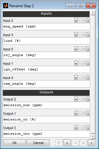
4.4 Rename inputs / outputs
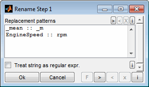
By default the names and units of the channels loaded are displayed besides the axes. Especially if many axes are displayed these names may lead to overlapping axes labels. Therefore you can rename the channels in a two step procedure (F2).
In the first step you will be asked for replacement patterns. These are applied to all channels and are useful to do common renaming tasks. The replacement patterns are given one rule per line. The string to look for and the replacement are separated by two colons, like "EngineSpeed :: rpm". The replacement is case sensitive and done in the order of lines from top to bottom. If the corresponding check box is set the strings are interpreted as regular expression.
In the second step you will be asked for each channel individually to modify the name and / or unit.
4.5 Order inputs / outputs
The display order of the inputs and outputs can be adjusted even after loading the data and training models. The order just influences the display and does not effect the model or optimization. By selecting the same order number for multiple outputs they will share the same axis. In contrast the order numbers of the inputs must be unique.
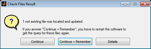
4.6 Check files
The files data was loaded from is remembered and will be used e.g. to prefill the dialog when reloading data. They can also be displayed using the data info (Ctrl + Shift + i).
It may happen that files have been renamed or moved during the work or after reloading a session. Use the “Check files” option in this case to search the missing files and update their names and path automatically. Remember that sometimes it is not possible to find missing files. Especially all files must be located in the same directory. The option “Continue + Remember” allows you to save search results and apply them quickly next time without prompting. To reset these saved replacements, the software must be restarted or the corresponding option must be used when the message after automatic replacement is displayed.
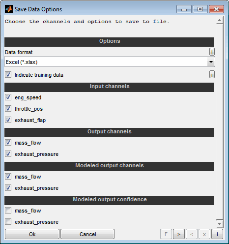
4.7 Save data
Also the saving of data points in different file formats is supported.
The storable data consists of the loaded data and the model values at the inputs of the loaded data. In this way, for example, data cleaned from outliers and interpolated model data can be stored (Ctrl + s). It is also supported to save an additional channel indicating the training data.
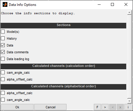
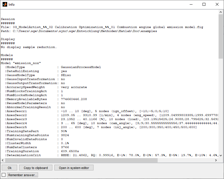
4.8 (Data) Info
You can display some information about the models and loaded data (Ctrl + Shift + i) like file names, comments, data loading / model history and calculated channels. This may be helpful to document the work done. Remember that the model quality information like RMSE represent the status after model training. Reloading the data, removing outliers will change this quality status but the information from the Data Info will not get updated.
Calculated channels will be shown by opening them in the CalcGuide. This is just for display purpose. Modifications done in the CalcGuide will be discarded. The data can be copied to the clipboard. In order to be able to find calculated channels quickly but also to be able to view the sequence of the calculation, they are displayed unsorted and sorted.
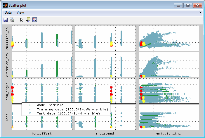
4.9 Scatter plot
Scatter plots enable to visualize relations between arbitrary inputs and outputs based on the training / test data and the model axes grid points. This helps to judge the loaded data and to detect outliers.
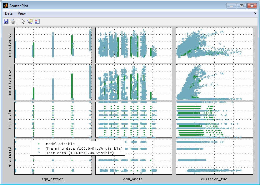
Data and model grid points shown are the ones that are allocated inside the actual axes ranges in the main window. So you can influence the scatter plot section by using the zoom functionality in the main window. Additionally when the scatter plot was created for the global operating point it will update automatically when the cursor positions in the main view are changed. For automatic updates the feature must be enabled in the menu of the scatter plot.
The following options will be asked when creating a scatter plot.
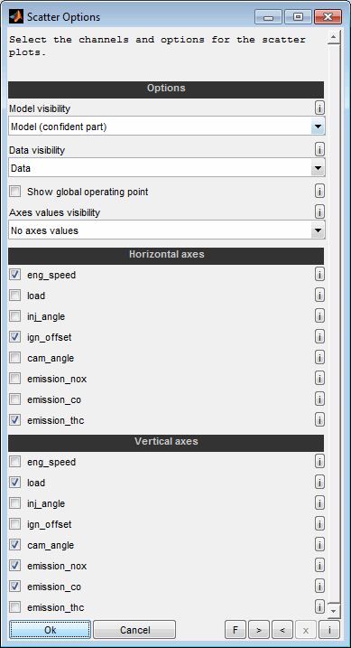
Model visibility
Using the model data for the scatter plot includes the advantages in data quality by the smoothness of the model and removed outliers. But you need to check the plausibility of the result especially in extrapolated model sections.
The model data shown is the one that is located inside the actual axes ranges in the main window. So you can influence the scatter plot section by using the zoom functionality in the main window. Additionally the scatter plot can be reduced to only show data for the actual global operating point in case only model data is visualized.
No optimization is done or considered. The granularity of data will be given by the breakpoints defined during model training. Therefore the axes must be chosen carefully and adequate finely graduated to create a significant scatter plot.
Model (entire)
The entire model data (axes grid points) will be shown in the scatter plot. Using the model includes the advantages in data quality by the smoothness of the model and removed outliers. But you need to check the plausibility of the result especially in extrapolated model sections. Outside the training data range the models may produce courses that look plausible but are impractical for the calibration system to reproduce - this behavior is usually undesirable. See the next option for an alternative to avoid the behavior.
Model (confident part)
The part of the model data (axes grid points + output values) inside the confidence limit will be shown in the scatter plot. Therefore the extrapolated model sections are not considered. The limit to judge a model to be confident can be edited using the “Edit model” feature.
Data visibility
The data points shown is the one that is located inside the actual axes ranges in the main window. So you can influence the scatter plot section by using the zoom functionality in the main window. The relative number of visible data points is shown in the legend.
No optimization is done or considered. The granularity of the data will be given by the data loaded. Therefore the data must be adequate finely graduated to create a significant scatter plot.
Data
The loaded data points used for model training will be shown in the scatter plot.
Show at global operating point
The scatter plot can be reduced to only show the data for the actual global operating point. If this option is selected the axes of the global inputs are interpolated at the actual values defined by the cursor positions. So you can create the scatter plot for an individual global operating point by setting the cursors of the global channels in the main window.
This option is only available when all data presented in the scatter plot is based on the models. So the “Data visibility” must be “None”. In case data should be visualized a reduction to the global operating point can be achieved by adjusting the main intersection view using the zoom functionality.
Horizontal / vertical axes
Choose the input / output data channels to consider for the scatter plots. For each combination of horizontal and vertical axes a scatter plot will be generated. If you would like to generate only specific combinations you can create multiple scatter plots sequentially.
Data subset indication
Subsets of the data points can be marked and colored. This can be done just for visualization and data analysis or as a preliminary work for the outlier removal – see the following section for details. The synchronized view of the data subsets supports the correlated judgment of the single scatter plots and additionally allows to establish a connection to their input values if both axes of a scatter plot are outputs.
By using the mouse you can mark single data points or rectangular sections. Afterwards you will be asked to choose a color for the subset. Since subsets are managed related to their color you can create discontinuous subsets by multiple selection when assigning a common color.
By selecting a subset in a scatter plot the cursors will be positioned at the mean value of the input values of the subset.
Data subset synchronization
Data subsets will be synchronized between the single plots. So when creating a subset in a scatter plot you will recognize the subset also in the scatter plots of other outputs, the correlation plots, the error plots and the Pareto plots. The subset also will be displayed in the intersection plots. By selecting a subset in a scatter plot the cursors will be positioned at the mean value of the input values of the subset. See “Data subset indication / synchronization” for details.
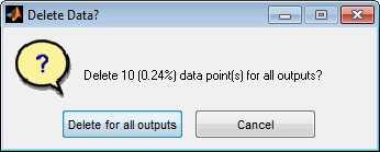
Data / outlier removal
Using the corresponding menu items or keyboard shortcuts data points can be removed. Before they must be combined in one or more data subsets. Then the selected or all subsets can be removed. Usually this feature is used to remove outliers from model training.
After closing the error plot window you will be remembered to retrain the model to adjust to the modified data.
4.10 Input / Output correlation plot
The data correlation visualizes the correlation between arbitrary inputs and outputs based on the training / test data points. This helps to quickly judge the relevance of the single inputs regarding the outputs (sensitivity analysis) and to identifying dependencies of the inputs.
The correlation values are in the range 0 to 1. 0 means no correlation and 1 perfect correlation. The displayed correlation coefficients are statistical values incl. their 95% confidence bounds. They provide a first indication of the interactions of the signals. In general, a low correlation between the inputs and a high correlation between the inputs and outputs is desired.
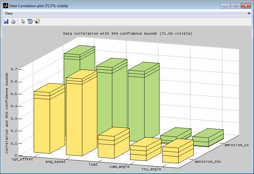
The data points regarded for calculating the correlation are the ones that are allocated inside the actual axes ranges in the main window. So you can influence the correlation plot section by using the zoom functionality in the main window. For automatic updates the feature must be enabled in the menu of the scatter plot.
The following options will be asked when creating a data correlation plot.
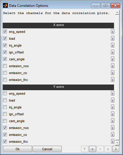
Axes
Choose the input / output data channels to consider for the data correlation plot. For each combination of x- and y-axes a correlation will be visualized. If you would like to generate only specific combinations you can create multiple data correlation plots sequentially.
4.11 Reduce data
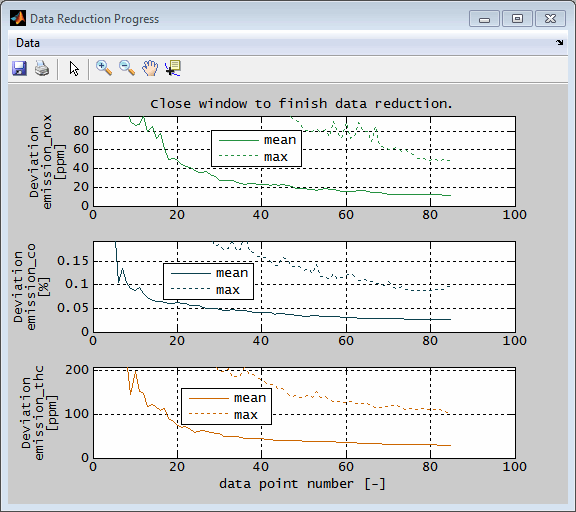
The data reduction feature enables to reduce the current data points in a way that preserves the model quality in the best or generates a spacefilling distribution. This can be for example used to speed up e.g. model training or system optimization.
Starting from a few points, data points are constantly added and the progress (quality of the resulting models or spacefilling distance criterion) is visualized. You decide how much you want to reduce the data based on this progress from the complete models or data points.
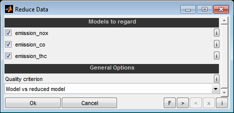
Models to regard
Choose whether to regard this model for data reduction quality. Only the models selected here will be used to determine the most suitable data points. All other models will be ignored.
Quality criterion
Select the quality target to be used for data reduction.
Model vs reduced model
The deviation of the original model based on all data points compared to the reduced data model is optimized. This prevents inaccurate measurement data from gaining weight as a result of data reduction. It is assumed that in case of inaccurate measurement data the actual model is accurate by averaging several data points.
Data vs reduced model
The deviation of all data points themselves from the reduced data model is optimized. The prerequisite for this is that the measurement data are very accurate. Otherwise, data reduction will make inaccurate data more important.
Data (spacefilling DoE)
The data points are considered solely on the basis of their distribution in relation to the inputs. The aim is to achieve the best possible distribution in the parameter space of the inputs. No model quality is taken into account and therefore no models must be selected in this case. Therefore, choosing the number of data points is less easy than with criteria based on model quality. The progress view visualizes the mean and minimum relative distance averaged over the points.
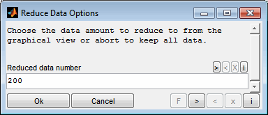
During data reduction, the progress is continuously displayed. When a model based quality criterion was selected the mean and maximum deviation for all selected models is displayed. When a spacefilling distribution was requested the relative mean and maximum distance of the points is visualized. When you are satisfied with the progress, close the window. The number of data points to be used is then queried. Use the graphic representation to choose an axis value that represents a good compromise between the number of points and the quality of the models or the spacefilling distribution. It is no problem to run the calculation longer than finally selected. The selected number of data points can lie in the entire section already processed.
The elected data amount is finally applied. means that only this number of most suitable data points is retained. All other data points are removed. The models remain unchanged. If the models are to be adapted to the reduced data, they must be retrained afterwards.
5 View
5.1 Zoom, pan, reset view
By zooming and paning the axes ranges one can quickly adjust the view to the relevant data. This does also influence the display of the data points inside all other plots, see Data point display.
The following techniques assist the view adjustment:
Zoom
Simply by dragging with the mouse inside any plot the axes ranges can be adjusted the scale in input and output direction.
Pan
Simply by dragging with the right mouse button inside any plot the axes ranges can be adjusted range in input and output direction.
Reset view
By resetting the view (Ctrl + F12, Ctrl + r) all input and output axes ranges are reset to fit the data and model (if any).
Reset act. x/y axis
By resetting the actual x/y axis (Shift + a) only the axes of the last clicked plot are reset. As all plots share the range of the input / output channels also plots with the same input / output channel are adjusted.
Fit all y-axes
This does quickly adjust all output axes ranges to fit the data without modifying the input axes (Ctrl + a).
Set axes range manually
You can manually set the axes ranges and tick width (Ctrl + x, Double click axes).
Undo / Redo
Using undo / redo functionality recent view configurations can be quickly restored (Ctrl + z, Ctrl + y).
5.2 Cursors
For each input channel a cursor is displayed. The cursor can be moved by dragging it with the mouse. While moving the actual axis value is displayed as well as the model value if any. Together all cursors define the actual input value set. This is used to determine the visibility and color of the data points regarding the max. distance criterion. See Data point display for further information.
5.2.1 Snap to data
If “Snap to data” is activated in the menu the cursors will always place themselves on the nearest data point.
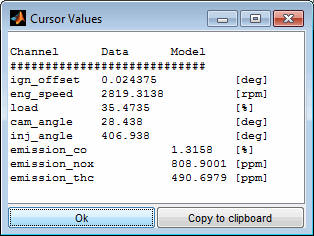
5.2.2 Copy cursor
The actual input values at the cursor locations can be visualized and copied to clipboard. Output values from the data points are only copied when all cursors match the same data point – this is quite rare, because each cursor can be located at any data point.
When a model is trained also the output values of the model are shown.
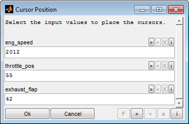
5.2.3 Set cursor position
To place the cursors at dedicated input value positions use the corresponding menu item or double click a cursor line. The input value positions must be within the range of the data points or model axes.
5.3 Element visibility
5.3.1 Toggle element visibility
Data points
The visibility of the data points in general can be turned on or off (Ctrl + d). The visibility of the single data points is determined regarding the max. distance criterion. See the following section. The color (Shift + Enter) and marker size of the data points can be modified. Model lines and the corresponding data points share the same color.
Model
The visibility of the model (if any) can be turned on or off (Ctrl + m). The visibility of the 95% confidence bounds can be toggled separately. The line width and color can be adjusted. Model lines and the corresponding data points share the same color.
Inputs / Outputs
The visibility of the inputs (Ctrl + 1..9) / outputs (Shift + 1..9) can be turned on or off column wise / row wise. At least one input and one output must remain visible. Be aware that the axis range and cursor position of invisible axes does influence the data point display of the remaining axes.
5.3.2 Data point display
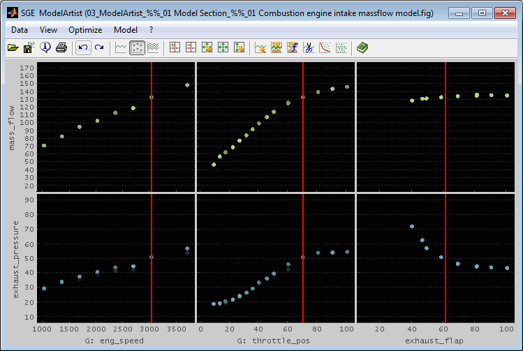
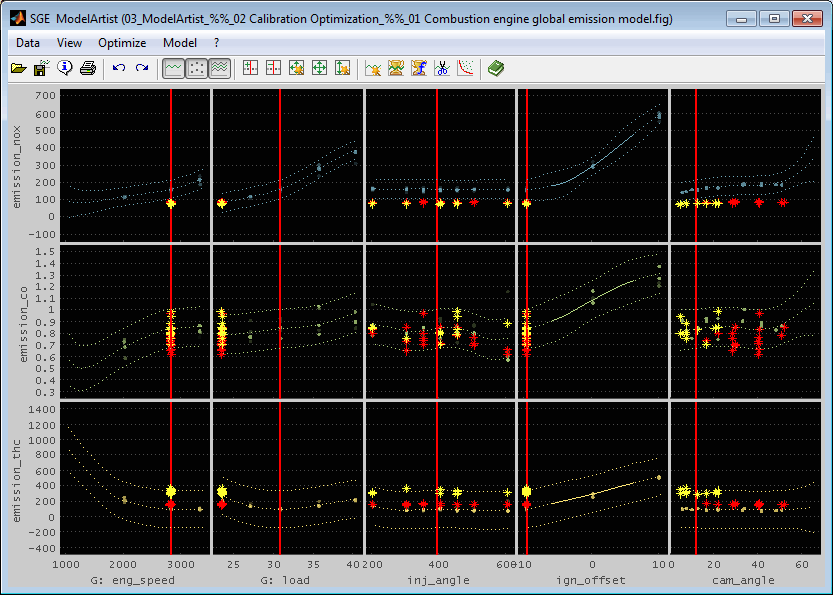
Usually a measurement consists of a number of single measurement samples. These are displayed as single points then. When all points are displayed this would look like in the following figure. One can hardly judge the input – output correlations.
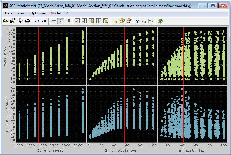
There are two ways to reduce and emphasize the data points to illustrate the correlations.
Zoom
Simply by dragging with the mouse inside any plot the axes ranges can be adjusted in input (and output) direction. As the data points displayed are the same for all plots and they must fit into the section of all input axes to be displayed, zooming is a suitable way to reduce the data points.
If an axis reduces the data points inside the other plots it is displayed colored red.
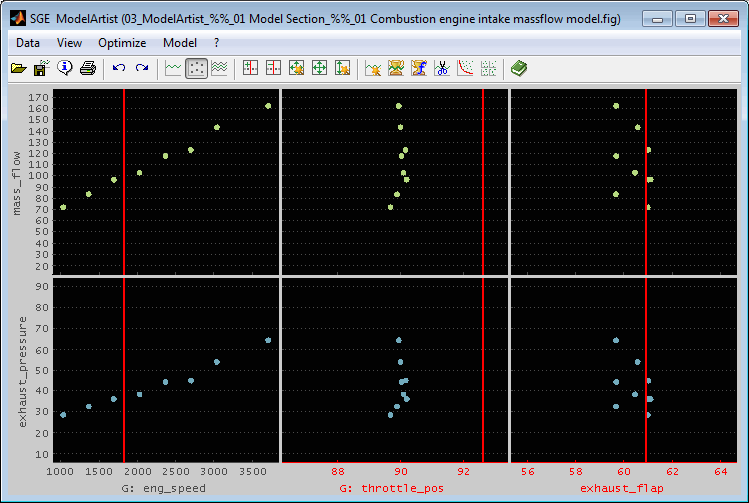
The following figure shows the previous figure with the throttle_pos and exhaust_flap axis zoomed. This reduces the data points in the plots with n_eng axes to this throttle section.
Max. data distance
The visibility of the data points is set in relation to its "data distance". This is the maximum of its distance to the actual cursor positions for all inputs except for the one of the plot itself. The more far the points are from the cursor positions the more invisible they get.
So for example to color the data points in the plots with n_eng axis the distance of their throttle position values to the cursor position in the throttle position axis is regarded.
Modify the data distance to influence the part of data to display. In the menu a max. data distance can be set. Data points exceeding this distance are colored completely black and are therefore invisible. The distance value is relative to the unzoomed axes ranges. Keyboard shortcuts can be used to quickly adjust the max. data distance (Ctrl + +/-).
In the following figure the max. data distance is set to 10% and therefore the left plots show the input – output correlation for about 70% throttle_pos and 60% exhaust_flap (right cursor values) and accordingly the right plots reduce their data with respect to the left cursor values.
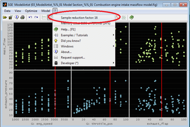
5.3.3 Automatic display reduction
To accelerate the display a sample reduction factor is used by default. It is automatically adjusted according to the performance of the computer. The actual display reduction value can be identified in the ?-menu.
Keyboard shortcuts can be used to quickly adjust the sample reduction factor (Ctrl + shift + + / - / F12). Changing the display reduction manually does turn off the automatic adjustment.
5.4 Data subset indication / synchronization
Subsets of the data points can be marked and colored in the correlation, error, Pareto and scatter plots. This can be done just for visualization and data analysis or as a preliminary work for the outlier removal.
By using the mouse you can mark single data points or rectangular sections. Afterwards you will be asked to choose a color for that subset. Since subsets are managed related to their color you can create discontiguous subsets by multiple selection when assigning a common color. In the correlation plots creating a subset can additionally be performed in relation to the error of the data points – see “Correlation plot” for details.
It is possible to mark data and model points. In this case you will be asked which ones should be processed to a subset.

Data subset synchronization
Data subsets will be synchronized between the single plots. So when creating a subset in an e.g. correlation plot you will recognize the subset also in the correlation plots of other outputs, the error plots, the Pareto plots and the scatter plots. The subset also will be displayed in the intersection plots. By adding a subset the cursors will be positioned at the mean value of the input values of the subset.
The synchronized view of the data subsets supports the correlated judgment of the single plots and additionally allows to establish a connection between the plots that may be solely based on output values (correlation plot, Pareto plot, scatter plot) and their input values. In the following figures the synchronization of the representation of two data subsets selected in the Pareto plot (red / yellow colored points) is illustrated.
Edit data subsets
In the "Data" menu of plots containing data subsets, the subsets can be reset or deleted. Reset only means that the points are no longer highlighted in color. Delete means that the corresponding data points are actually removed. Deleting is only possible for data points and not model points. When deleting subsets of model points, they are ignored. Depending on the context, data points can be deleted for the current or all outputs.
Reset and delete is provided for the selected or all data subsets. To select a data subset, you can mark it with the mouse.

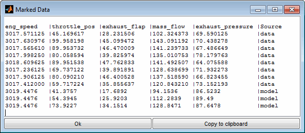
Copy data subsets
In case data subsets are marked they can be visualized in a numeric view and also copied to clipboard using the corresponding menu items or keyboard shortcuts (Ctrl + c). For each data or model point a line will be included containing the values of all inputs and outputs and additionally a “Source” column showing whether its a data or model point. Using the “Copy to clipboard” button copies the data into the clipboard in a format that can be inserted in e.g. a spreadsheet software.
5.5 Color, Marker size, Line width
The color of the model line and data points can be modified for each output separately. Additionally the marker size and line width can be influenced. Use the corresponding menu items to access these features.
5.6 Background color
Using the corresponding menu item enables to adjust the background color of the intersection plots.
5.7 Window arrangement
Since the ModelArtist offers to open a considerable number of windows (e.g. correlation, error, Pareto, scatter plots) an automatic window arrangement feature is implemented. Using the corresponding menu item enables to arrange all or a subset of the windows of the current session.
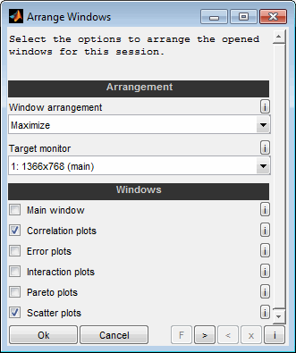
Window arrangement
Select the layout of the arrangement. It is possible to maximize, minimize, restore or close all selected windows. Additionally column and row based layouts are available.
Example: "2-3 of 5 rows" means that the screen is split into 5 rows and the second and third row is used for the layout.
Target monitor
Select the target monitor for the windows to arrange in case of multiple monitors are connected to the computer.
Windows
Select which windows to include into the arrangement. It is not allowed to close the main window. So in case the arrangement is “close” it is not allowed to select the main window.
6 Model
6.1 Train model
From the data loaded a model can be trained (Ctrl + Shift + m). This model can then be used for optimization or just to visualize scattered data in a homogeneous way.
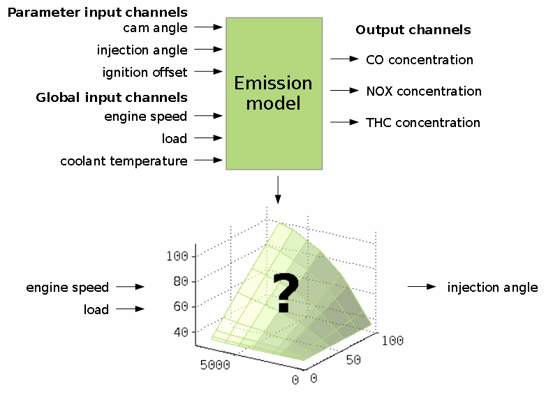
A model predicts some output channel values based on input channel values. The output channel values are the optimization targets. They will be minimized or maximized. There are two types of inputs channels. Parameter input channels are tuning factors to optimize the output channels values. Global channels define e.g. the operating point and will not be judged as a variable value to optimize the outputs.
A typical example is an emission model as shown in the following schema.
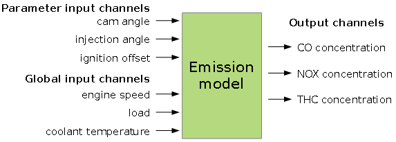
Selecting the model type, axes and options has significant influence on the ability to fit the data course. Consult the help corresponding to the single input fields and this manual. Always judge the result using the correlation and error plots.
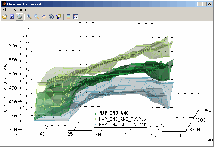
The model is displayed as a line. The line style is continuous inside the confidence limit. Outside the confidence limit the line style of the model is a dotted line when the model type supports confidence information. In this case also the 95% confidence bounds (= two times the standard deviation) can be displayed as dotted lines. The displayed confidence bounds always show the 95% confidence interval. The editable confidence limit determines the solid/dotted display of the model itself. See “Edit model” for details.
Each output has a individual model. Not all outputs necessarily need to have a model. All models trained in one run will have the same model type. If you need different model types for some outputs you need to run model training for the outputs separately.
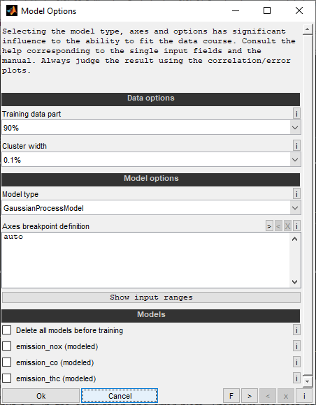
Training data part
Select the part of the data loaded to use for model training. This part is called training data. The rest of the data is called test data and will not be regarded during model training but e.g. in the correlation and error plots. Therefore the test data allows a better judgment of the model prediction quality. Keep in mind that the amount of test data reduces the training data accordingly.
Cluster width
Clustering enables to concentrate the input data by means of an adjustable tolerance. All points whose input values are within the tolerance are combined to form a single point for modeling by forming the mean value of each input and output value. This reduces the data point number for the model training and combines repeated measurement points to reduce their tolerance.
Zero disables the clustering and higher values mean an increasing concentration of the data points. The tolerance refers to the value ranges of model axes and data points of the individual input channels. For an input with a model axis from 1000 to 10000 and data points from 500 to 9500 this means that 1% tolerance refers to the range 500 to 10000 and is thus 95.
Use small values (e.g. 0.1%) if unsure.
Model types
Different types of models to train are available. The model types differ regarding ability to fit data courses and training speed. Always use the error plots available after model training to judge the quality of the model fit.
Model axes
You will also be asked to define the axes breakpoints of the models to train.
Enter an axes definition for each model input - one per line. The number of lines must match the input number. Alternatively you could enter only one line which then will be used for all inputs.
The axes breakpoints can be defined by just entering a scalar numeric value for the breakpoint number. In this case the breakpoints will be equally distributed in the range of the data values of the input. If you put only one line, it is considered for all inputs, if more lines are applied they must match the input number and are applied to the corresponding input. Alternatively you could enter an explicit breakpoint definition or enter "auto" for automatic breakpoint selection.
Example 1:
6 → Equally spaces axes with 6 breakpoints for all inputs.
Example 2:
auto → Automatically determine breakpoint number and values.
6 → Equally spaces axes with 6 breakpoints (input 1).
0 2000 4000 8000 → Explicit definition of axis (input 2).
0:2000:10000 → Explicit definition of equally spaced axes (input 3).
linspace(0,10000,20) → Explicit definition of equally spaced axes (input 4).
Select a suitable breakpoint number / definition considering the following factors:
When performing a calibration optimization the optimized parameter input values (except for the input to calibrate) will be a axes breakpoint member. So the accuracy of the optimization will be given by the breakpoints defined during model training. Therefore axes of parameter input channels to optimize must be chosen carefully and adequate finely graduated.
When performing a calibration system optimization with the data source “Model” the model grid values will be used and therefore optimization will only be performed for these values. So the result of the optimization will be influenced by the breakpoints defined during model training. Therefore axes of input channels must be chosen carefully and adequate finely graduated.
When creating a Pareto plot it will only consist of the model grid members. Therefore axes of input channels must be chosen carefully and adequate finely graduated. Also scatter plots may contain model data.
When a model is exported it will be converted to an n-dimensional grid where n is the number of inputs. The grid axes will be the model axes. So the granularity of the grid will be given by the breakpoints defined during model training. Therefore the axes must be chosen carefully and adequate finely graduated and e.g. concern the later usage of the export (e.g. interpolation method). Some interpolation methods provide no extrapolation and therefore outside the axes ranges NaN values will be generated.
For data visualization little breakpoint numbers often are sufficient because the model lines shown will be drawn by an algorithm generating a smooth course. The error plots available are the appropriate medium to judge the quality of the model fit.
High breakpoint numbers in case of many inputs may slow down the GUI after model training. During model training high breakpoint numbers may lead to a lot of calculation effort.
After axes definition a visualization of the axes distribution and the data points will be displayed. When the axes do not include all data points a warning message will be generated. The message also indicates the data range necessary for full data coverage.
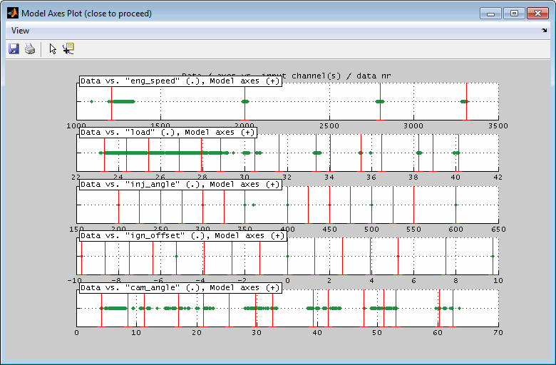
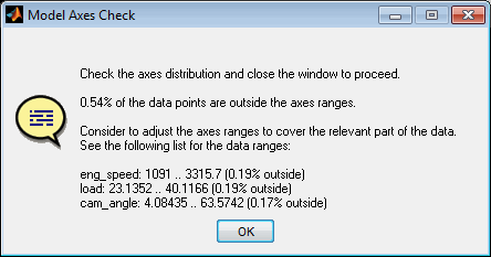
Selecting the model axes has significant influence on the ability to fit the data course. Always judge the result using the correlation and error plots. Especially the error plots are very useful when judging the suitability of the axes chosen. See the corresponding section ”Error plot” for details.
6.2 Edit model
Some model properties are editable after model training.
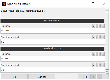
Bounds
Enter the min/max bounds to limit the model to separated by spaces. Remember that applying bounds cannot be undone. You need to retrain the models to remove the bounds applies.
Examples:
"0 100" -> Lower limit 0, upper limit 100.
'"0 inf" -> Lower limit 0, no upper limit.
"-inf 100" -> No lower limit, upper limit 100.
Confidence Limit
Specify a limit for the variance of the model within which the model is considered to be confident. Specify a scalar value >= 0 in the unit of the output.
The limits refers to the 95% confidence interval of the model. This data is available for some model types and enables to judge the confidence of the model values. The model part with a 95% confidence interval not exceeding this limit will be jugded to be confident. This confidence criterion is used for several features and also the model display. The confident part will be display as a solid line in the intersection plot. The rest is displayed as a dotted line.
Examples:
65
6.3 Model quality judgment
To judge the correlation of the model values vs. the measured values and therefore the model quality different views are available.
Especially for Gaussian process models it is essentially important to use these views to detect and remove outliers from the data points and retrain the models afterwards.
6.3.1 Model training result
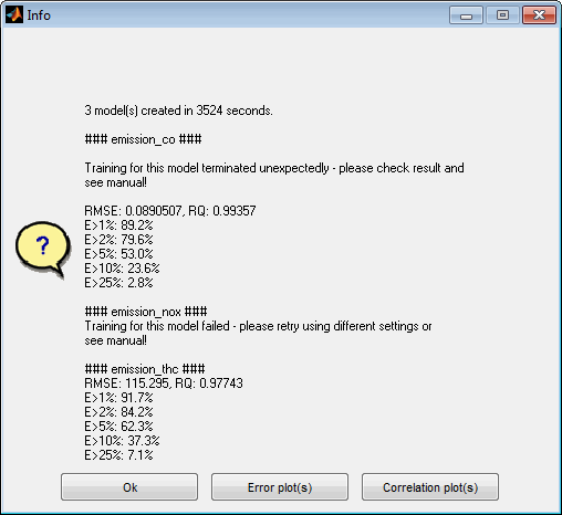
After completing the model training a result will be displayed that summarizes information regarding the archived model qualities. For each model trained the root mean square error and the determination coefficient are shown as well as the data parts exceeding certain error levels. The message also allows to directly show the corresponding error or correlation plots.
In case of unexpected training events a hint will be shown and it is recommended to check the model thoroughly and retrain as required with different settings. In case of Gaussian process models you could for example try another model type or use transformations.
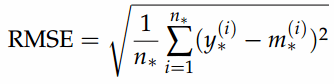
The root mean square error is explained in the following formula where y* are the data values, m* the model values and n* the number of data values.
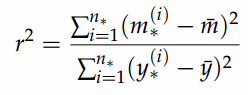
The determination coefficient is explained in the following formula where y* are the data values, m* the model values, y is the mean value of all data values, m the mean value of all model values and n* the number of data values.
Generally spoken the RMSE is the much more robust and reliable error criterion and is a good starting point for model judgment.
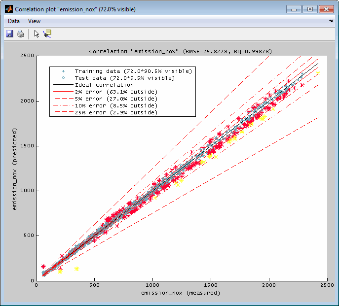
6.3.2 Correlation plot
A correlation plot can be displayed for every output separately. It contains a representation of the output values of the data points (x-axis) and their model values (y-axis). The ideal correlation and some standard error lines are available. The data points shown are the ones that are allocated inside the actual axes ranges in the main window. So you can influence the correlation plot section by using the zoom functionality in the main window – if this feature is enabled in the menu of the correlation plot. The relative number of visible data points is shown in the legend and the window title.
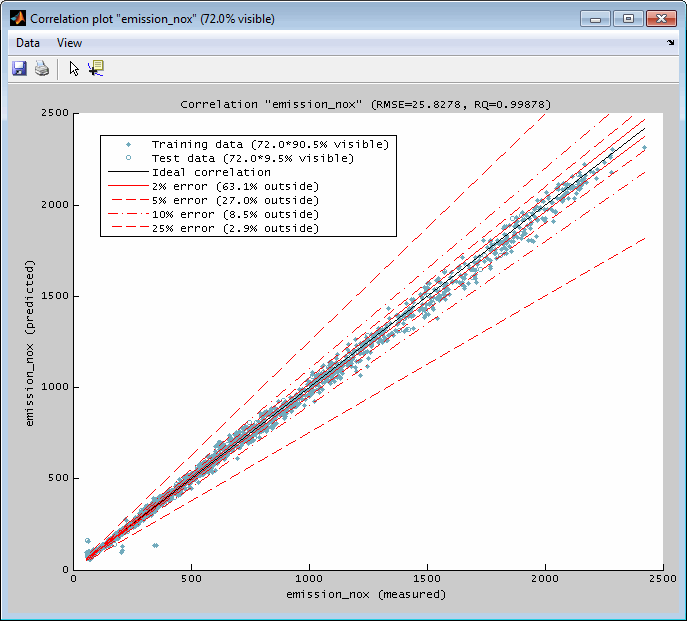
The correlation plot also informs about the root mean square error and the determination correlation criterion. The view can be adjusted using zoom and reset functionality – available by menu items or keyboard shortcuts.
Data subset indication
Subsets of the data points can be marked and colored. This can be done just for visualization and data analysis or as a preliminary work for the outlier removal – see the following section for details.
By using the mouse you can mark single data points or rectangular sections. Afterwards you will be asked to choose a color for the subset. Since subsets are managed related to their color you can create discontiguous subsets by multiple selection when assigning a common color.
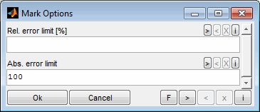
Creating a subset can additionally be performed in relation to the error of the data points. This can be done by specifying a relative of absolute error limit.
Data subset synchronization
Data subsets will be synchronized between the single plots. So when creating a subset in a correlation plot you will recognize the subset also in the correlation plots of other outputs, the error plots, the Pareto plots and the scatter plots. The subset also will be displayed in the intersection plots. By selecting a subset in a correlation plot the cursors will be positioned at the mean value of the input values of the subset. See “Data subset indication / synchronization” for details.
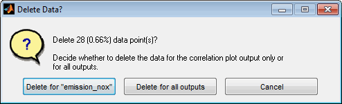
Data / outlier removal
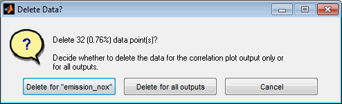
Using the corresponding menu items or keyboard shortcuts data points can be removed. Therefore create one or more data subsets. Then the selected or all subsets can be removed. Usually this feature is used to remove outliers from model training.
When removing outliers you will be asked whether to remove them only for the output related to the correlation plot or for all outputs. In case the outlier is caused by e.g. the measurement system of the output it is sufficient to remove it only for this output. If e.g. the input measurement was affected by some inaccuracy it may be necessary to remove it for all outputs.
The decision is assisted by the synchronized view of the data subsets. When opening all correlation plots at the same time the subset used for outlier removal can be judged easily to see whether multiple outputs are affected or only the actual one.
After closing the correlation plot window you will be reminded to retrain the model to adjust to the modified data.

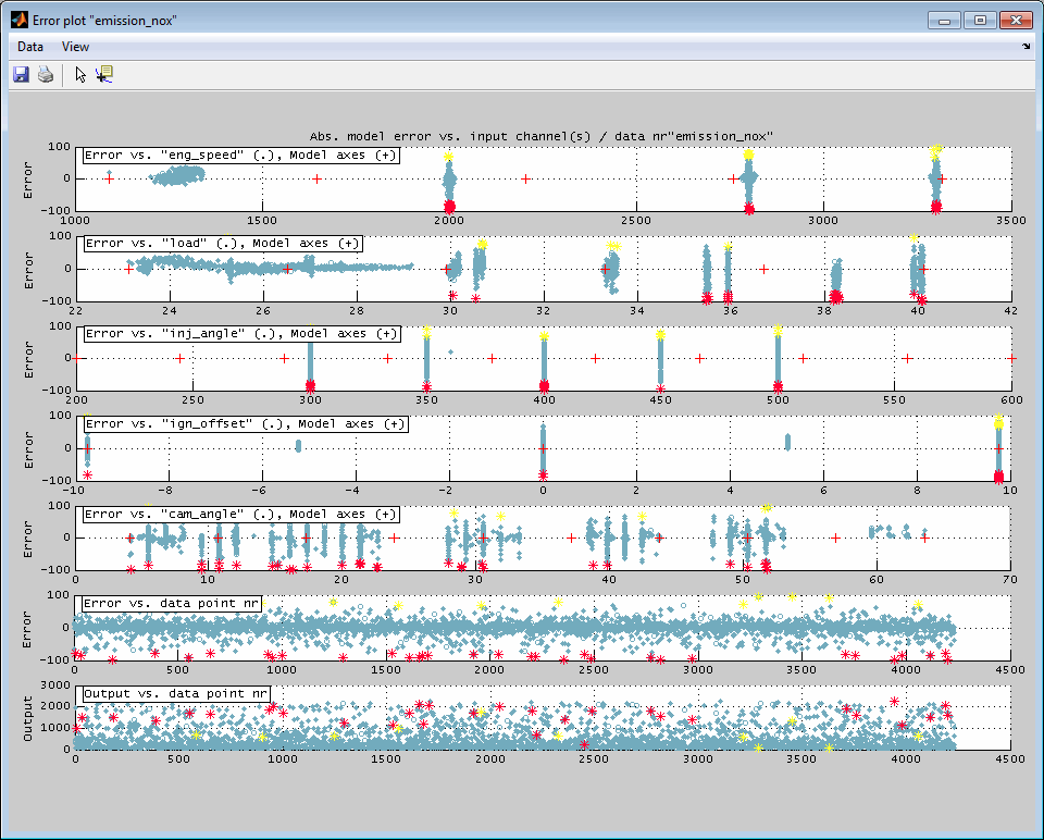
6.3.3 Error plot
A representation of the model error (y-axis) related to every input (x-axis) separately can be displayed. This helps to judge the location of the model error related to the inputs and may be useful to adjust the model axes. The view additionally contains a plot of the model error and model output values related to the data point number which may help to detect drifts or varying data inaccuracy during data acquisition.
The error plot is generated for each output separately.
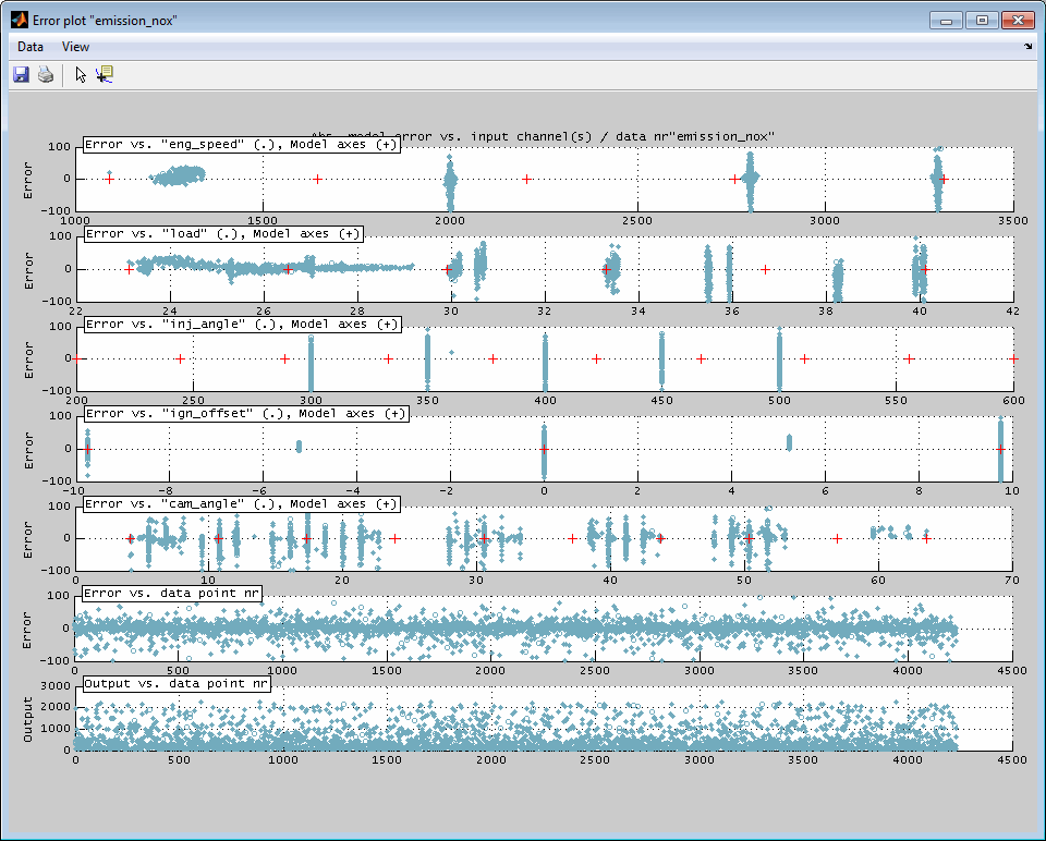
The data points shown are the ones that are allocated inside the actual axes ranges in the main window. So you can influence the error plot section by using the zoom functionality in the main window – if this feature is enabled in the menu of the error plot.
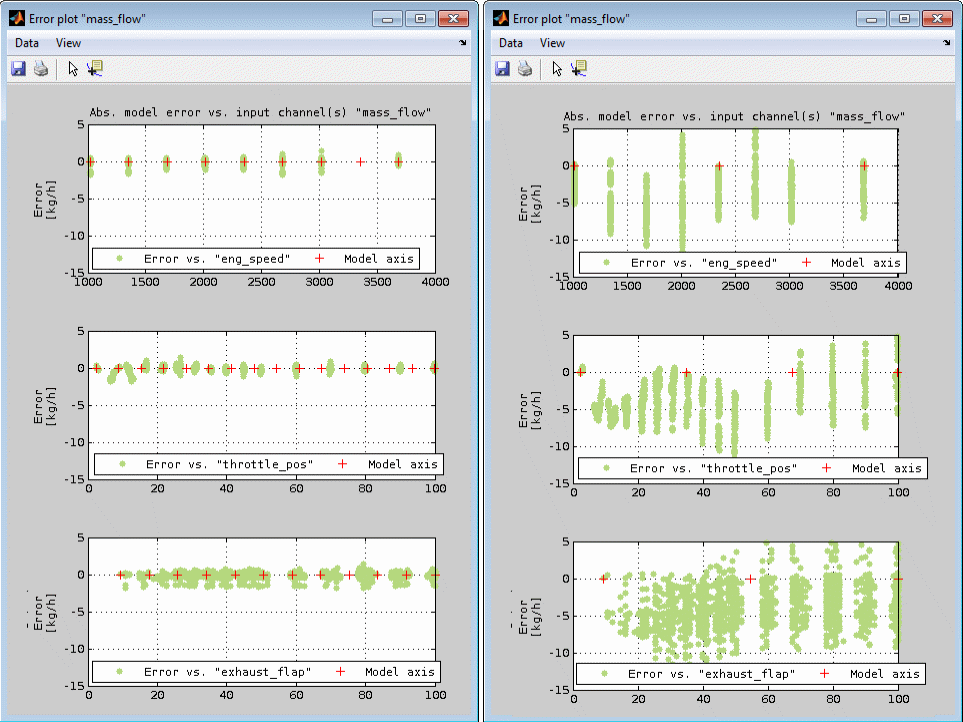
Model axes judgment
The following figure shows an example of the influence of the axes chosen for model creation to the model fit. On the left side the model axes are sufficiently fine spaced and located which results in only little error for all inputs while on the right side the too rare axes breakpoints lead to a drastically increasing model error.
Data subset indication
Subsets of the data points can be marked and colored. This can be done just for visualization and data analysis or as a preliminary work for the outlier removal – see the following section for details.
By using the mouse you can mark single data points or rectangular sections. Afterwards you will be asked to choose a color for the subset. Since subsets are managed related to their color you can create discontinuous subsets by multiple selection when assigning a common color.
Data subset synchronization
Data subsets will be synchronized between the single plots. When creating a subset in an error plot you will recognize the subset also in the error plots of other outputs, the correlation plots, the Pareto plots and the scatter plots. The subset also will be displayed in the intersection plots. By selecting a subset in an error plot the cursors will be positioned at the mean value of the input values of the subset. See “Data subset indication / synchronization” for details.
Data / outlier removal
Using the corresponding menu items or keyboard shortcuts data points can be removed. Before they must be combined in one or more data subsets. Then the selected or all subsets can be removed. Usually this feature is used to remove outliers from model training.
When removing outliers you will be asked whether to remove them only for the output related to the error plot or for all outputs. In case the outlier is caused by e.g. the measurement system of the output it is sufficient to remove it only for this output. If e.g. the input measurement was affected by some inaccuracy it may be necessary to remove it for all outputs.
The decision is assisted by the synchronized view of the data subsets. When opening all error plots at the same time the subset used for outlier removal can be judged easily to see whether multiple outputs are affected or only the actual one.
After closing the error plot window you will be reminded to retrain the model to adjust to the modified data.
6.4 Pareto plot
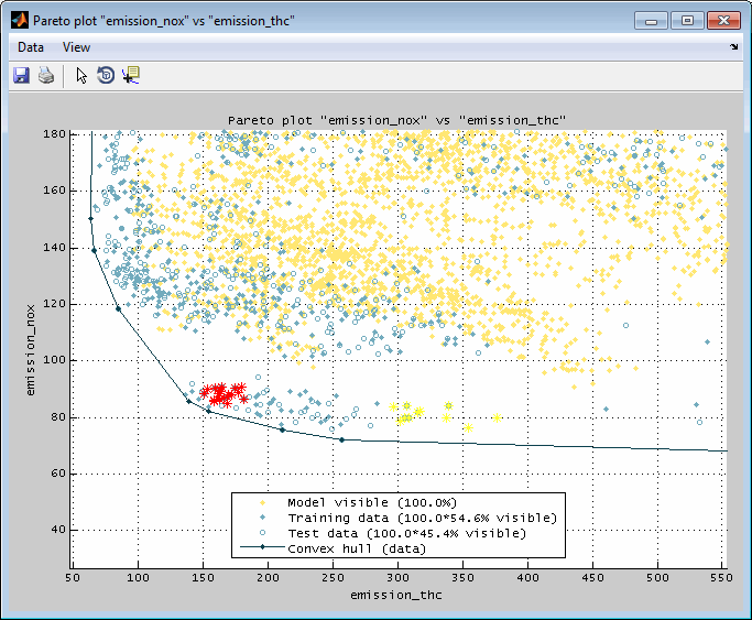
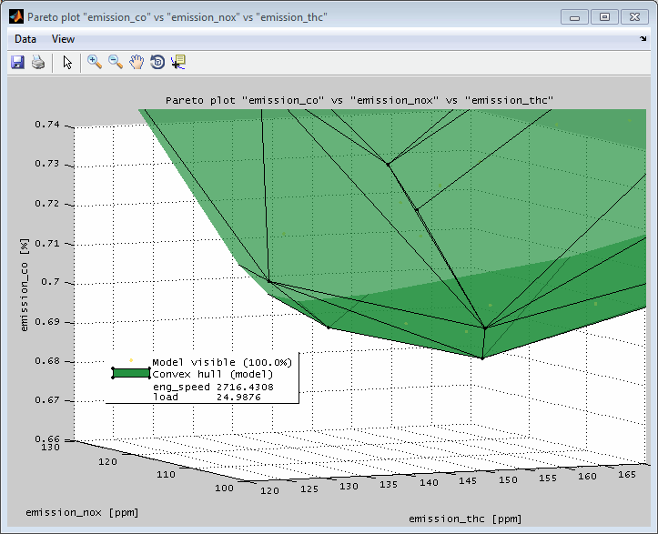
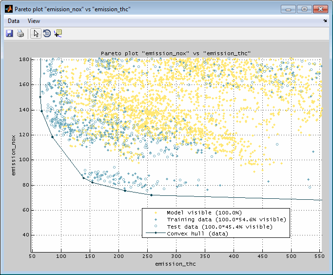
The Pareto plot shows the relation of two or three model outputs. It allows to judge a state in which it is not possible to improve one output without having to simultaneously degrade another. A typical example would be different emission components or fuel consumption vs emissions.
The data and model grid points shown are the ones that are allocated inside the actual axes ranges in the main window. So you can influence the Pareto plot section by using the zoom functionality in the main window. Additionally when the Pareto plot was created for the global operating point it will update automatically when the cursor positions in the main view are changed. For automatic updates the feature must be enabled in the menu of the Pareto plot.
In the following example the trade off of some emission components is shown for a combustion engine. In the 2D view the model grid points are shown and surrounded by a convex hull. Additionally the training and test data points are included. In the 3D view only model grid points are shown for a single global operating point. The hull is representing the Pareto front and allows the judgment of the influence on an output if the other one is optimized.
The following options will be asked when creating a Pareto plot.
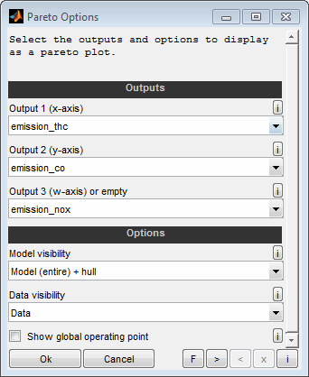
Outputs
Select the model outputs to display on the single axes of the Pareto plot. You can select two or three outputs. Leave empty the third input to create a 2D graphics and choose all three outputs to create a 3D graphics. If the Pareto plot will be based on model data the axes grid of the model selected for “Output 1” will be used to retrieve the axes grid values for all outputs related in the Pareto plot.
So for example you could select three emission components to visualize the trade off between these components when optimizing them separately.
Model visibility
Using the model data for the Pareto plot includes the advantages in data quality by smoothness of the model and removed outliers. But you need to check the plausibility of the result especially in extrapolated model sections.
The model data shown is the one that is located inside the actual axes ranges in the main window. So you can influence the Pareto plot section by using the zoom functionality in the main window – if the feature is enabled in the menu of the Pareto plot. The relative number of visible data points is shown in the legend. Additionally the Pareto plot can be reduced to only show data for the actual global operating point in case only model data is visualized.
No optimization is done or considered. The granularity of the data will be given by the breakpoints defined during model training. Therefore the axes must be chosen carefully and adequate finely graduated to create a significant Pareto plot.
Model (entire)
The entire model data (axes grid points) will be shown in the Pareto plot. Using the model includes the advantages in data quality by the smoothness of the model and removed outliers. But you need to check the plausibility of the result especially in extrapolated model sections. Outside the training data range the models may produce courses that look plausible but are impractical for the calibration system to reproduce - this behavior is usually undesirable. See the next option for an alternative to avoid the behavior.
Model (confident part)
The confident part of the model data (axes grid points + output values) will be shown in the Pareto plot. The limit to judge a model to be confident can be edited using the “Edit model” feature.
Model hull…, … + hull,
If selected the model points are surrounded by a convex hull or only the hull is displayed. Depending on the shape the hull may be representing the Pareto front and allows the judgment of the influence to an output if the other one is optimized. Since the hull is created of surfaces it is usually easier to judge its shape compared to the points on their own.
Data visibility
The data points shown is the one that is located inside the actual axes ranges in the main window. So you can influence the Pareto plot section by using the zoom functionality in the main window – if the feature is enabled in the menu of the Pareto plot.. The relative number of visible data points is shown in the legend.
No optimization is done or considered. The granularity of the data will be given by the data loaded. Therefore the data must be adequate finely graduated to create a significant Pareto plot.
Data
The loaded data points used for model training will be shown in the Pareto plot.
Data hull…, … + hull
If selected the data points are surrounded by a convex hull or only the hull is displayed. Depending on the shape the hull may be representing the Pareto front and allows the judgment of the influence to an output if the other one is optimized. Since the hull is created of surfaces its usually easier to judge its shape compared to the points on their own.
Show at global operating point
The Pareto plot can be reduced to only show the data for the actual global operating point. If this option is selected the axes of the global inputs are interpolated at the actual values defined by the cursor positions. So you can create the Pareto plot for an individual global operating point by setting the cursors of the global channels in the main window – if the feature is enabled in the menu of the Pareto plot.
This option is only available when all data presented in the Pareto plot is based on the models. So the “Data visibility” must be “None”. In case data should be visualized a reduction to the global operating point can be achieved by adjusting the main intersection view using the zoom functionality.
Data subset indication / synchronization
Subsets of the data points can be marked and colored. Data subsets will be synchronized between the single plots. So when creating a subset in a Pareto plot you will recognize the subset also in the correlation plots and the error plots. The subset also will be displayed in the intersection plots.
The synchronized view of the data subsets supports the correlated judgment of the single Pareto plots and additionally allows to establish a connection to their input values. Therefore trade off selections in the Pareto plot can be evaluated regarding their input value settings. See “Data subset indication / synchronization” for details.
By using the mouse you can mark single data points or rectangular sections in 2D Pareto plots. In 3D Pareto plots you can select single points of the data or hull. Afterwards you will be asked to choose a color for the subset. Since subsets are managed related to their color you can create discontiguous subsets by multiple selection when assigning a common color. When marking sections containing model and data points at a time only the model points will be considered to create a subset.
By selecting a subset in a Pareto plot the cursors will be positioned at the mean value of the input values of the subset.
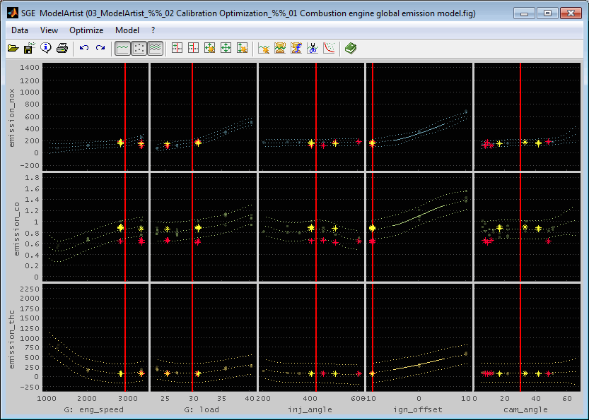
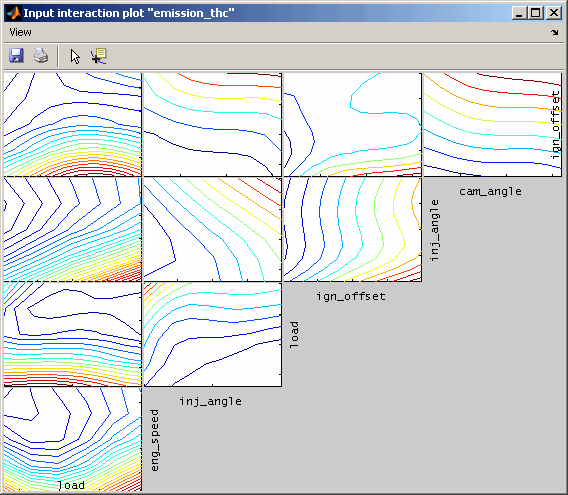
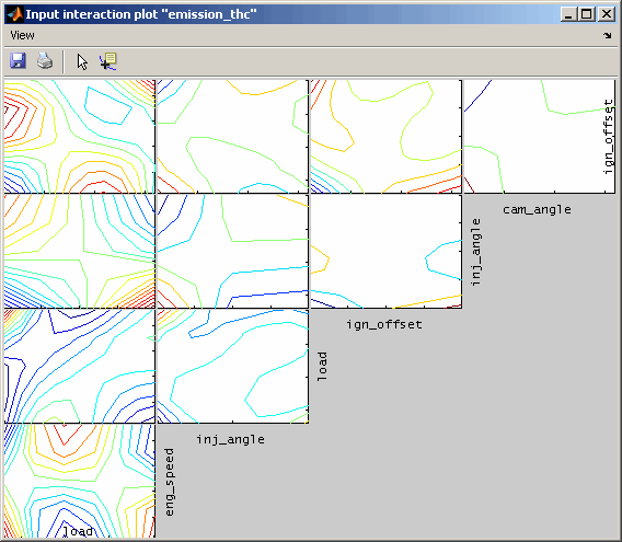
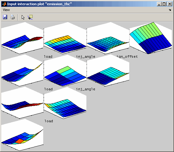
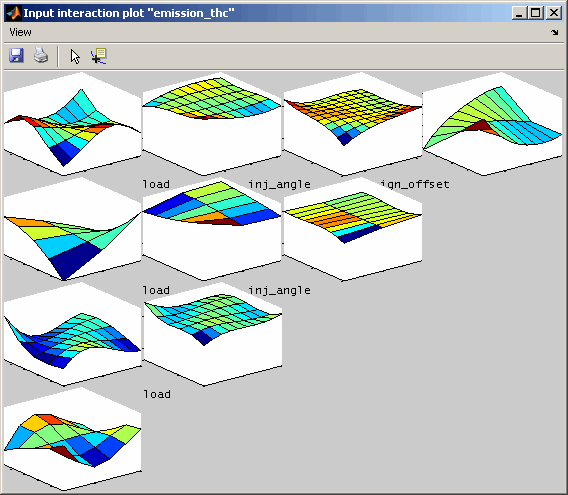
6.5 Input interaction plot
Input interaction plots visualize for each input channel combination the output or confidence interval of the model. All other input values result from the actual cursor settings. When the cursor in the intersection plot is moved, the input interaction plots will be updated – if this feature is enabled in the menu.
The following options are available:
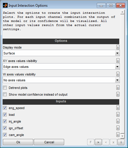
Display mode
You can select whether to display the interaction plots as surface or contour representation.
Axes values visibility
You can select whether and how to display axes values.
Detrend plots
When selected the interaction plots will be detrended. This means that influences of one input that does not depend on the other input, is removed. Thus, the maps shown are flatter and better to judge.
Show model confidence instead of output
When selected the interaction plots will show the model confidence interval instead of the model output directly. This feature enables to locate sections of the model with poor confidence.
Inputs
Choose the input data channels to consider for the interaction plot.
The following figures show the interaction plots for one output. On the left side the unmodified results are compared to the detrended ones the right side.
6.6 Model export
Models can be exported to different formats.
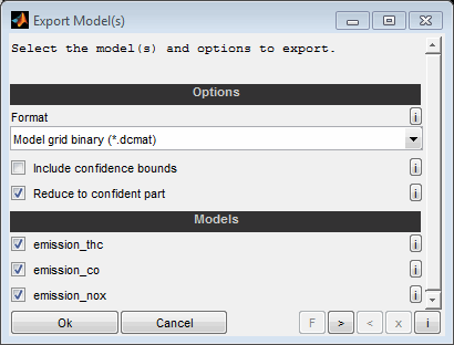
Format
See the following sections for details regarding the available formats to export.
Include confidence interval
The 95% confidence interval may also be exported if supported by the model type.
Reduce to confident section
Decide whether the export should be reduced to the model part with sufficient confidence. Sections outside this range will be set to invalid (NaN). The limit to judge a model to be confident can be edited using the “Edit model” feature.
6.6.1 Model grid export
When a model is exported (Ctrl + e) it will be converted to an n-dimensional grid where n is the number of inputs. So for example a model with two inputs will generate a map, with three inputs a cube and so on. The grid axes will be the model axes. So the granularity of the grid will be given by the breakpoints defined during model training. Therefore the axes must be chosen carefully and adequate finely graduated and e.g. concern the later usage of the export (e.g. interpolation method). Some interpolation methods provide no extrapolation and therefore outside the axes ranges NaN values will be generated.
The following formats are available to export models to:
Model grid (*.cdfx)
The models can be exported to a CDF file This is a ASAM standard calibration parameter format similar to DCM format files and can be used in an external software. For example it can serve as interpolation object in a calculated channel. Thus it is possible to calculate model output for arbitrary input values. The ASAM standard supports up to 5 inputs. Anyway if a model has more than 5 inputs it may be exported.
Model grid binary (*.dcmat)
For models with high number of inputs and axes breakpoints you may experience problems when saving and loading the file to *.cdfx format. Use the binary (*.dcmat) format in this case. Since it is no standard format you can use it only within the SGE Circus tools and MATLAB/Simulink. See “Model usage in Simulink“ for details.
MATLAB function (*.m)
This format saves an *.m file for each output that can be used within MATLAB to calculate the model output. See “Model usage in MATLAB” for details.
6.6.2 Model list export
Alternatively models can be exported (Ctrl + e) as a list of the grid points in different file formats. This results in a data file containing the model grid points sequentially and may be for example suitable for map creation.
In case all models exported share the same grid axes the target file will contain these axes only once. Otherwise the axes will be exported separately for the single models. Therefore the target file format chosen must support separate axes.
6.6.3 Model usage in Simulink
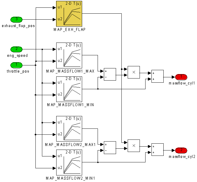
A model grid exported as a DCMAT file is adequate to use the model in MATLAB/Simulink. You can use an “Interpreted MATLAB Fcn” block or an “n-D Lookup Table” block in Simulink.
Interpreted MATLAB Fcn
The “Interpreted MATLAB Fcn block” enables to interpolate the models with only little manual interaction but it is not suitable for code generation. Make sure to adjust the configuration at the beginning of the file and of the Simulink block according to the requirements.
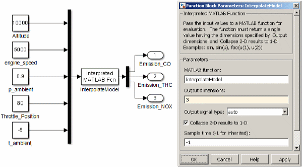
Save the following function to a file called InterpolateModel.m in the Matlab search path and follow the instructions at the beginning of the file.
% #####################################################################
% # SGE InterpolateModel #
% # Use ModelArtist model grid export (*.dcmat file) in Simulink #
% #####################################################################
%
% SGE Ingenieur GmbH
% 05.11.2017
%
% This function is intended to interpolate a ModelArtist model grid export
% from a *.dcmat file in Simulink using a "Interpreted Matlab Fcn" block.
% Save this file to a path available in Matlab / Simulink and make sure
% to adjust the Configuration section at the beginning.
%
% Set the block parameters in Simulink and connect the inputs to a bus creator
% that concatenates as many signals as model inports.
%
% Block parameters:
% Output dimensions: Number of labels in "LabelNamesModel" configuration
% for scalar input. In case of vector inputs enter the
% total number of data samples.
% "1" for one label, "2" for two labels (scalar input)
% MATLAB function : "InterpolateModel"
%
function[out] = InterpolateModel(in)
% ############# Configuration ################
% Label names of models grid inside DCMAT file
LabelNamesModel = {'Model_CUBE_5_BrakePower','Model_CUBE_5_BrakePower'};
% DCMAT file
LabelFile = 'Condor_20160418_GT_ModelSession_AllOutputs_ModelExport_power.dcmat';
% Interpolation method
InterpolationMethod = 'linear'; % linear, nearest, pchip, cubic, spline
% Extrapolation method
ExtrapolationMethod = 'none'; % none (=NaN), linear, nearest, pchip, cubic, spline
% Replacement value for NaN interpolation result (outside axes range)
NanReplacementValue = 0;
% ######## End of configuration ##############
persistent ticLastRun GriddedInterpolant
% Check if file exists
if ~exist(LabelFile,'file')
error('File does not exist: %s',LabelFile);
end
% Check label format
if ~iscell(LabelNamesModel)
error('Configuration "LabelNamesModel" must be a cell of label name strings.');
end
% Load file. Reuse data if last run was recently.
if isempty(ticLastRun) || toc(ticLastRun) > 0.1
try
FileData = load(LabelFile,'-mat');
catch err
error('Error loading file: %s',err.message);
end
% Data included
if ~isfield(FileData,'CalibrationDataStruct')
error('File does not contain "CalibrationDataStruct" (%s).',LabelFile);
end
% Create persistent gridded interpolants for for single labels
for iL = 1:length(LabelNamesModel)
% Search for label
LabelIndex = find(strcmp(FileData.CalibrationDataStruct.LabelNames,LabelNamesModel{iL}),1);
if isempty(LabelIndex)
error('Label "%s" not found in file "%s".',LabelNamesModel{iL},LabelFile);
end
% Get label data
Label = FileData.CalibrationDataStruct.LabelW{LabelIndex};
AxX = FileData.CalibrationDataStruct.LabelX{LabelIndex};
AxY = FileData.CalibrationDataStruct.LabelY{LabelIndex};
% Must be numeric
if ~isnumeric(Label)
error('Label must be numeric and not of class "%s".',class(Label));
end
% Create interpolant
if isscalar(Label)
GriddedInterpolant{iL}.Type = 1;
GriddedInterpolant{iL}.NumInputs = 0;
GriddedInterpolant{iL}.Interpolant = Label;
elseif isvector(Label)
GriddedInterpolant{iL}.Type = 2;
GriddedInterpolant{iL}.NumInputs = 1;
GriddedInterpolant{iL}.Interpolant = griddedInterpolant(AxX,Label,InterpolationMethod,ExtrapolationMethod);
elseif ismatrix(Label)
GriddedInterpolant{iL}.Type = 3;
GriddedInterpolant{iL}.NumInputs = 2;
GriddedInterpolant{iL}.Interpolant = griddedInterpolant({AxX,AxY},Label,InterpolationMethod,ExtrapolationMethod);
else
GriddedInterpolant{iL}.Type = 4;
GriddedInterpolant{iL}.NumInputs = ndims(Label);
GriddedInterpolant{iL}.Interpolant = griddedInterpolant([{AxX},AxY(:)'],Label,InterpolationMethod,ExtrapolationMethod);
end
end
end
% Dimension check
if GriddedInterpolant{1}.Type == 1
if ~isempty(in)
error('Input must be empty for a scalar parameter.');
end
end
% Initialize result
out = cell(length(LabelNamesModel),1);
% Reshape input in case of input vectors
if GriddedInterpolant{1}.NumInputs > 2
in_act = num2cell(reshape(in,numel(in)/GriddedInterpolant{1}.NumInputs,GriddedInterpolant{1}.NumInputs),1);
end
% Loop for single labels
for iL = 1:length(LabelNamesModel)
% Perform interpolation
if GriddedInterpolant{iL}.Type == 1
out{iL} = GriddedInterpolant{iL}.Interpolant;
elseif GriddedInterpolant{iL}.Type == 2
out{iL} = GriddedInterpolant{iL}.Interpolant(in_act);
else
out{iL} = GriddedInterpolant{iL}.Interpolant(in_act{:});
end
% Check for valid output. No NaN or inf allowed in Interpreted Matlab fcn
out{iL}(isnan(out{iL}) | isinf(out{iL})) = NanReplacementValue;
end
clear iL
% Create matrix from cell
out = [out{:}];
ticLastRun = tic;
end
n-D Lookup Table
The “n-D Lookup Table” block enables to interpolate the models and also supports code generation. But some manual interaction is required to setup. Make sure to adjust the configuration at the beginning of the file and of the Simulink block according to the requirements.
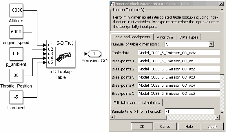
Save the following function to a file called ModelExport2Workspace.m in the Matlab search path and follow the instructions at the beginning of the file. The file must be executed before simulation and code generation to make the model data and axes available in the MATLAB workspace. The variable names are generated automatically and must be inserted into the block configuration. Use the MATLAB command “who” to retrieve the variable names after executing the function.
% #####################################################################
% # SGE ModelExport2Workspace #
% # Export ModelArtist model grid export (*.dcmat file) to workspace #
% # for usage in LoopUp Table blocks. #
% #####################################################################
%
% SGE Ingenieur GmbH
% 04.06.2019
%
% This function is intended to export a ModelArtist model grid export
% from a *.dcmat file to Matlab workspace for usage in Simulink in
% LoopUp Table blocks.
% Save this file to a path available in Matlab / Simulink.
%
% Set the block parameters in Simulink to adjust the label names and dimension.
%
function[] = ModelExport2Workspace()
% Load file
[File,Path] = uigetfile('*.dcmat','Select ModelArtist Export File');
if isequaln(File,0)
return;
end
LabelFile = fullfile(Path,File);
% Load file
FileData = load(LabelFile,'-mat');
% Data included
if ~isfield(FileData,'CalibrationDataStruct')
error('File does not contain "CalibrationDataStruct" (%s).',LabelFile);
end
% Find models names
ModelNames = {};
for i=1:length(FileData.CalibrationDataStruct.LabelNames)
if isnumeric(FileData.CalibrationDataStruct.LabelW{i}) && ~isempty(regexp(FileData.CalibrationDataStruct.LabelNames{i},'^Model_','once'))
ModelNames(end+1) = FileData.CalibrationDataStruct.LabelNames(i); %#ok
end
end
[~,SortInds] = sort(lower(ModelNames));
ModelNames = ModelNames(SortInds);
if isempty(ModelNames)
error('No models found in file: %s',LabelFile);
end
% Select models
[IndsSelected,Ok] = listdlg('ListString',ModelNames,'PromptString','Select Models To Transfer To Workspace','SelectionMode','multiple');
if ~Ok || isempty(IndsSelected)
return;
end
LabelNamesModel = ModelNames(IndsSelected);
% Remember names
WorkspaceNames = {};
for iL = 1:length(LabelNamesModel)
% Search for label
LabelIndex = find(strcmp(FileData.CalibrationDataStruct.LabelNames,LabelNamesModel{iL}),1);
if isempty(LabelIndex)
error('Label "%s" not found in file "%s".\n\nAvailable labels: %s',LabelNamesModel{iL},LabelFile,strjoin(FileData.CalibrationDataStruct.LabelNames(:)',', '));
end
% Get label data
Label = FileData.CalibrationDataStruct.LabelW{LabelIndex};
AxX = FileData.CalibrationDataStruct.LabelX{LabelIndex};
AxY = FileData.CalibrationDataStruct.LabelY{LabelIndex};
% Must be numeric
if ~isnumeric(Label)
error('Label must be numeric and not of class "%s".',class(Label));
end
% Transform to target name and put to workspace
Name = [genvarname(LabelNamesModel{iL}) '_data'];
assignin('base',Name,Label);
WorkspaceNames{end+1} = sprintf('\n%s',Name); %#ok
if ~isempty(AxX)
Name = [genvarname(LabelNamesModel{iL}) '_ax1'];
assignin('base',Name,AxX);
WorkspaceNames{end+1} = sprintf(', %s',Name); %#ok
end
for iAx = 1:length(AxY)
Name = [genvarname(LabelNamesModel{iL}) '_ax' num2str(iAx+1)];
assignin('base',Name,AxY{iAx});
WorkspaceNames{end+1} = sprintf(', %s',Name); %#ok
end
end
% Report
fprintf('\n%d model(s) were transferred to the workspace. Each model consists of a data grid and axes vectors. These are suitable for usage in a Simulink n-D-lookup-table or the MATLAB interpn() function. The generated variable names are:\n%s\n',length(LabelNamesModel),strjoin(WorkspaceNames(:)',''));
end
6.6.4 Model usage in MATLAB
A model grid exported using the format “MATLAB function (*.m)” is adequate to use the model in MATLAB. It includes a MATLAB function that can be called using the filename as function name. The input parameters must be numeric vectors – one for each input of the model exported. All input parameter vectors must have same length. The output will be a column vector of identical length for the model output prediction. Additionally the confidence bounds can be retrieved as output parameters if they were exported.
See the header of the file for details calling the function. The following lines show a sample usage and remember that the *.mat file that is also created must be present for proper functionality.
[y_Predict, y_ConfidenceMin, y_ConfidenceMax] = exhaust_pressure(eng_speed, throttle_pos, exhaust_flap)
y_Predict = exhaust_pressure(eng_speed, throttle_pos, exhaust_flap)
6.7 Model import
Models can be imported from a CDF/DCM calibration parameter file. This is an ASAM standard calibration parameter format.
Curves, maps and parameter types with more than three dimensions can be loaded. The dimension of the parameters loaded must match the input number if data is already loaded. For example to load a map exactly two inputs must exist and to load a cuboid exactly three inputs must exist.
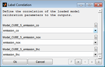
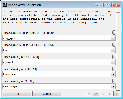
If more than one output exists or if more than one label is loaded you will be asked to correlate the parameters loaded to the output(s). To not assign any model to an output keep the corresponding field empty.
Afterwards you will be asked to assign the inputs to the axes of the parameters loaded. The axes ranges of the first parameter loaded are shown to ease the choice. The correlation will be used commonly for all parameters loaded. If the axes assignment of the parameters is not identical the import must be done sequentially for the single parameters.
6.8 Model section
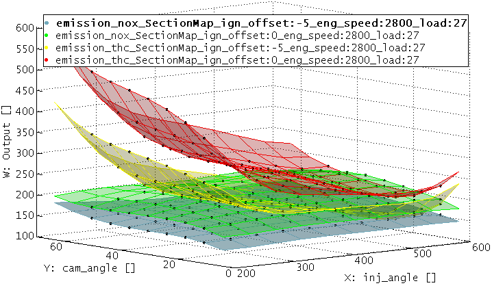
The dimension of a model matches its input number. A model section reduces the model dimension by setting some of its inputs to fixed values (Ctrl + t). The resulting section can have two, one or no inputs and therefore be a map, curve or a scalar value.
A model section is a quick way to get an illustrative representation of a part of the model. For example a model with five inputs can be reduced to two inputs and therefore just a map remains. A model section may be useful just for visualization purposes but also to derive calibration parameters. Creating a section for multiple models simultaneously allows to judge a model trade off.
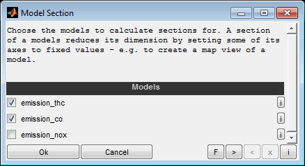
To create a model section first of all the models to derive sections from have to be selected. Afterwards the fixed input values and some options will be asked.
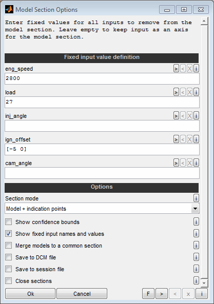
Fixed input value definition
For all input channels a scalar value can be entered to remove the corresponding axis from the model. Leave the field empty to keep the input as an axis of the model section. The scalar values must be within the range of the corresponding axis. The axis range can be received from the help of each individual input field.
To create multiple sections at once the fixed values can be specified to be vectors with more than one entry. In this case all input definitions must be vectors of same size or scalars.
Examples:
10 -> Set input to value 10.
[10 20] -> Create to section with values 10 and 20.Section mode
Decide how the section should indicate the area covered by data points. This way it is possible to judge which model areas are extrapolated.
Model (entire) : The entire model range will be shown in the section.
Model (confident part) : Only the confident part of the model will be shown. The limit to judge a model to be confident can be edited using the “Edit model” feature.
Model + indication points: The entire model range will be shown in the section and the confident section will be indicated by additional points. The limit to judge a model to be confident can be edited using the “Edit model” feature.
Show confidence interval
Decide whether the section should include the model 95% confidence interval.
Show fixed input names and values
Decide whether the section visualization should include the names and values of the fixed axes values.
Merge models to a common section
Select whether to create a common section view for all models. Otherwise each selected model section will create an individual view.
Save to calibration parameter file
Decide whether to save the section maps, curves and values to a calibration parameter file.
Save to session file
Select whether to automatically save the section views to session files. The file names will be generated automatically. Existing files will not be overwritten. If the ModelArtist session was already saved the sections sessions will be created in the same folder. Otherwise a target folder will be asked for.
Close sections
Select whether the sections should be closed automatically. This may be useful if a session or calibration parameter file was saved automatically.
Finally the resulting model section will be shown graphically. If selected, a dialog will be shown to save the model section and additional information to a calibration parameter file.
7 Optimize
7.1 Calibration parameter optimization
A model can be used to optimize calibration parameters. These are maps or curves that assign a z-value based on x/y-axes input values or scalars. Parameters to calibrate must have a model parameter input channel as z-value and global model input channels as axes values.
To pick up the emission model example a typical calibration parameter would be the injection angle map. Its axes engine speed and load are global input channels of the model and its z-value to calibrate (injection angle) is a parameter input channel of the model.
So the calibration optimization task would be to find for every map breakpoint combination the injection angle that leads to minimal CO emissions. If you like to optimize a criterion depending on multiple channels or need to regard constraints you may create a calculated channel as output to optimize. See section Multiple criteria optimization for details.
A calibration optimization returns a result only for one input channel at a time. This does not mean that the other channels are not optimized (see below) but the result will only be shown for one input. If you want to optimize multiple input channel calibration values this must be done sequentially. See Multiple parameter optimization for details.
7.1.1 Single parameter optimization
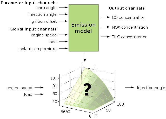
Starting the optimizing of a calibration parameters some options will be asked.
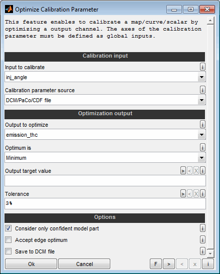
Input to calibrate
Select the input channel to calibrate. It must be the z-value of the parameter to calibrate.
Calibration parameter source
The parameter to calibrate can be retrieved from DCM/PaCo/CDF file or from ETAS INCA software. Therefore INCA must be started and an experiment must be opened. The parameter will be retrieved from the active calibration page.
The parameter may also be created as a standard map/curve/scalar value. In this case the axes are equally spaced with a range matching the model axes.
Output to optimize
Select the channel to optimize. If you like to optimize a criterion depending on multiple channels you have to create a calculated channel as output to optimize while loading data.
Optimum is
Select the optimization direction or "Target" to minimize the mean absolute difference of the output to a fixed value. The value is specified in the following input field.
Output target value
Enter a target value for the output to optimize. Enter a scalar numeric value. The absolute difference of the output to optimize from this value will be minimized. This option must be empty unless "Optimum is" is "Target".
Tolerance
Enter a tolerance for the output to optimize. The tolerance will be used to calibrate boundary maps. So additionally to the optimally calibrated parameter a minimum and maximum parameter will be calibrated to match the tolerance. This helps to afterwards smooth the parameter regarding the effect on the output to optimize. The value entered here can be relative or absolute. If the value ends with % it is regarded as relative in percent.
Consider only confident model part
If enabled only the confident part of the model will be considered for optimization. The limit to judge a model to be confident can be edited using the “Edit model” feature.
Accept edge optimum
If disabled, the optimum must not be at the edge of the value range of the input. This means that values must exist in both input directions which are poorer than the optimum.
If enabled, the optimum is allowed to be at the edge. The value is then not necessarily optimal but corresponds to the edge of the data area or the confidence area of the model and there is the possibility that even better results can be achieved beyond.
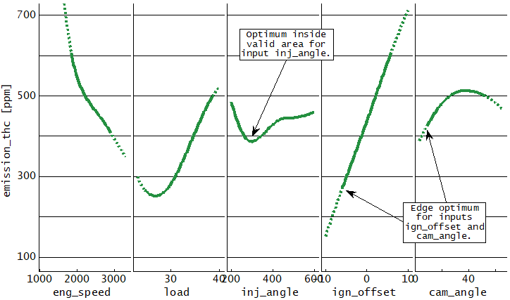
Save to calibration parameter file
The optimized maps, curves and values can be saved to a calibration parameter file.
Depending on the calibration parameter source chosen the DCM/PaCo/CDF file and parameter will be asked or the default map/curve/scalar value will be created.
Once the input channel to calibrate was chosen you have to decide how to handle the remaining parameter input channels. In our example these are the cam angle and the ignition offset.
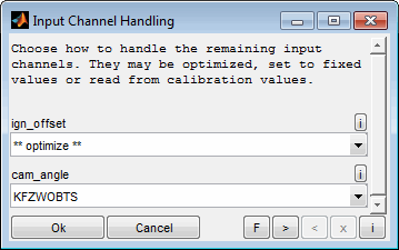
You may choose between the following alternatives:
**optimize**
The input channel will also be optimized. This will be done in the background and you will not be able to see the resulting values. Optimization will be done by selecting the optimum from the model axes values. Therefore during model training the axes must be chosen carefully regarding the granularity to enable effective optimization.
**fixed value**
The input channel will be set to a fixed value that will be asked afterwards.
** mean/min/max/std output selection **
All axes values of the input will take part in the optimization. The statistical calculation used to merge the correlating output values can be selected. So when you choose "mean output selection" the optimization will calculate the mean output value for all values of this input and optimize it. Also optimization of the maximum and minimum value is available as well as the standard deviation which may be used to prefer an constant output during optimization independent from its absolute value.
As an example the emission data was recorded for several engines and therefore the model will have an additional input “engine nr”. So the calibration optimization task would extend to find one common injection angle map that minimizes CO emissions for all engines. In this case we would typically choose “** max output selection **” to ensure that the maximum emission of all engines is minimized.
When multiple inputs use this mode they must use the same statistical calculation.
Calibration parameter
The input channel values will be retrieved from an already available calibration parameter. Imagine that the calibration for the ignition offset was already done and the parameter is available from the same source as the parameter to calibrate. In this case the parameter can directly be used and the input channel values will be calculated from the parameter. The parameter may be a map, curve or scalar calibration value. The axes of the parameter must be global input channels of the model. The available parameters are given by the source of the parameter to calibrate - e.g. a calibration parameter file or ETAS INCA software.
Then the axes of the parameters need to be assigned to global input values of the model. If at that time the input channels were not defined as global this may be done using the corresponding menu item without reloading the data.
If the calibration parameters were loaded from file the axes ranges will be shown to ease the channel assignment.
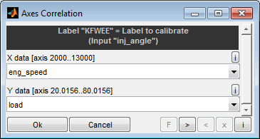
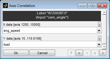
A model may have more global inputs than the calibration parameters axes number. In this case a fixed value for all not assigned global values will be asked. Also input channels may be set to fixed values (see above) that will be asked here. In our example the coolant temperature is defined as a global channel and will be asked as it is not an axis of the calibration map for the injection angle. Also the cam angle will be asked because we decided not to optimize it and not to read it from a already existing calibration parameter.
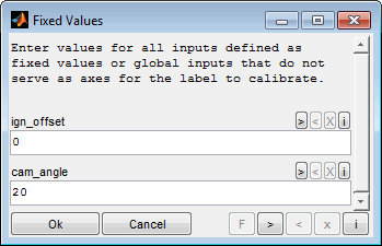
After supplying all needed input the calibration parameter is optimized. If a tolerance was given also the upper and lower boundary parameters will be created. A dialog will be shown to save the parameters and additional information to a calibration parameter file and the resulting parameters will be shown graphically. Scalar parameters will be displayed numerically.
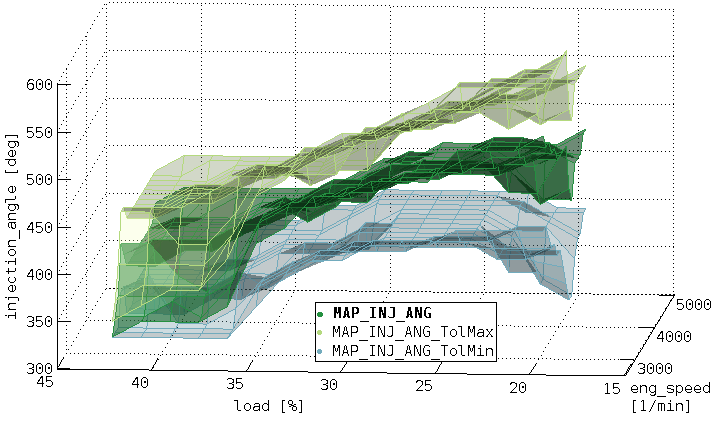
In case the parameters contain invalid values (NaN) you will be asked for a replacement value because invalid values cannot be written to a calibration parameter file. Leave empty to keep the invalid values.
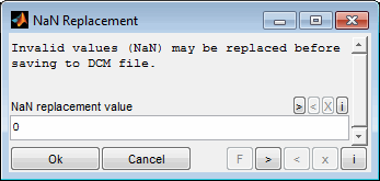
7.1.2 Multiple parameter optimization
A calibration optimization gives a result only for one input channel at a time. This does not mean that the other channels are not optimized but the result will only be shown for one input. If you want to optimize multiple input channel calibration values this must be done sequentially.
When the task is to optimize the injection angle and the ignition angle to minimize some emissions we would first select for example the injection angle for optimization. During this optimization we already set the handling for the ignition angle input to **optimize**. This will be done in the background and you will not be able to see the resulting values. Optimization will be done by selecting the optimum from the model axes values. Therefore during model training the axes must be chosen carefully regarding the granularity to enable effective optimization.
This way we retrieve a optimized injection angle map that can afterwards be smoothed and limited.
In a second step we repeat the optimization for the ignition angle map. This time we set the input handling for the injection angle input to use the already optimized map resulting from the first optimization. For the map to be available for selection it must be stored in the same source that is used to retrieve the ignition calibration parameter to optimize. When the source is set to DCP/PaCo/CDF file it must also contain the optimized injection angle map. When the source is set to ETAS INCA software the dataset must contain the optimized injection angle map.
The advantage of this approach is that the results of previous optimizations can already be taken into account for each optimization.
7.1.3 Multiple criteria optimization
Apart from the actual goal of optimization - thus minimizing a model output, you can consider other options such as boundary conditions or the weighting of different outputs by calculated channels.
Here are some examples:
Multiple channel optimization operating point independent
Here the three emission components are converted to a single mean value and at the same time normalized because of their widely different ranges of values. The result is a channel to use as model output to minimize with equal consideration all emission components – in the same manner for all global operating points.
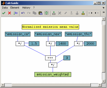
Multiple channel optimization operating point dependent
Here the three emission components are converted to a single mean value with operating point (speed, load) dependent weighting at the same time. The weighting is performed by maps, which are read from a calibration parameter file. It is also possible to specify the maps directly in the calculation ("InterpolMap" object).
The result is again a channel to use as model output to minimize. Thus, e.g. at higher loads the NOX are valued more, whereas at low loads, the other components are in the foreground.
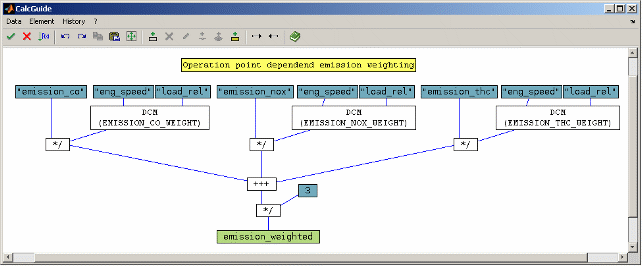
Constraints / limits
To consider boundary conditions can be realized by "punishing functions". In the following example, the CO emissions are increased by a factor depending on the exhaust gas temperature and misfiring rate. The factor is interpolated from curves that consist of an axis (for example, [800 850 900]) and a penalty factor (for example [1 1.1 2]).
By punishing the emissions the optimization will avoid optimization results where the constraints or limits are violated.
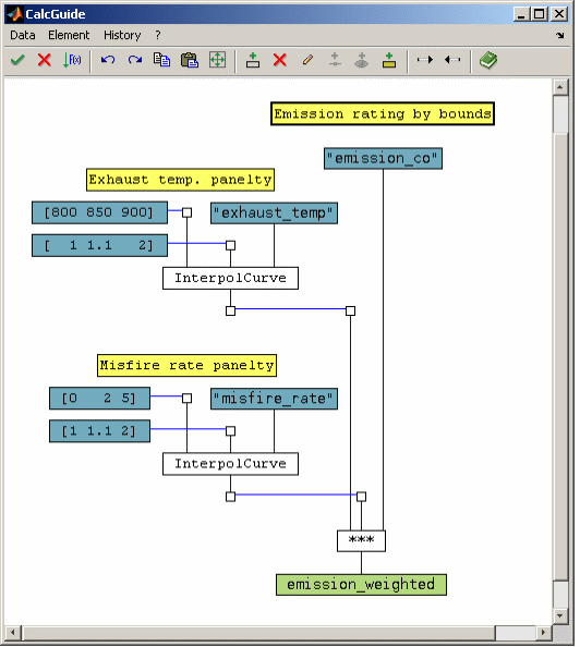
7.2 Calibration system optimization
Usually ECU function systems are physically based and include maps, curves and scalar calibration parameters that are connected using mathematical operations. This way they calculate an output value depending on some input values.
The calibration task is to find values for all parameters of an ECU system that minimize the deviation of the system output compared to reference values that are usually generated from measurement or simulation. This task might be very challenging because an ECU function cannot yet represent the correlations of arbitrary systems in a complete and real-time manner – e.g. internal combustion engines. Thus, often only main effects are implemented in a way that an entirely exact setting of the calibration parameters is no longer feasible and a compromise has to be made through prioritization. Additionally sometimes calibration parameters cannot be determined directly or not in the entire operating range. For example, Otto engine torque models or exhaust-gas temperature models often contain parameters which apply to 100% ignition efficiency and lambda one. If these operating ranges cannot be measured for reasons of knocking limits or component protection, only an indirect determination is possible.
The ModelArtist supports to automatically calibrate ECU systems (Ctrl + Shift + o) to match the ECU system behavior with one or more models or the loaded data points. This is done avoiding the mentioned problems and resolving the challenges and therefore provides the calibration engineer and software developer an universal tool for the automated calibration of ECU functions.
The following figure shows a typical ECU system to calculate the intake mass flow for two cylinders individually depending on engine speed, throttle position and exhaust flap position.
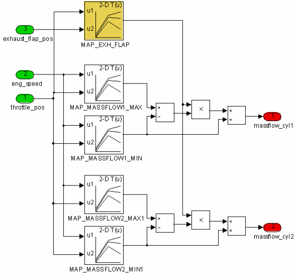
For each cylinder a minimum and maximum mass flow map exists and a central weighting map MAP_EXH_FLAP implements the exhaust flap influence. While the two mass flow maps could easily be calibrated by measurements the weighting map cannot. It has to balance the two cylinders and also the engine_speed influence, because the map itself has no engine speed input.
To perform a calibration system optimization first of all we create models to exactly describe the system behavior. The models have the same inputs and outputs as the ECU system. Though one model does have exactly one output we need two models – one for each cylinder. As usual the models are trained using measurement data. The following figure shows the models. As an alternative it is also possible to use just the loaded data points for optimization without need for any model.
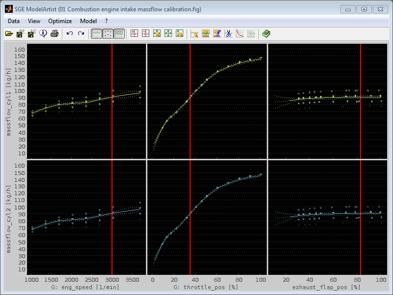
Then we can start the system optimization.
7.2.1 Settings
Starting a calibration system optimization some options will be asked.
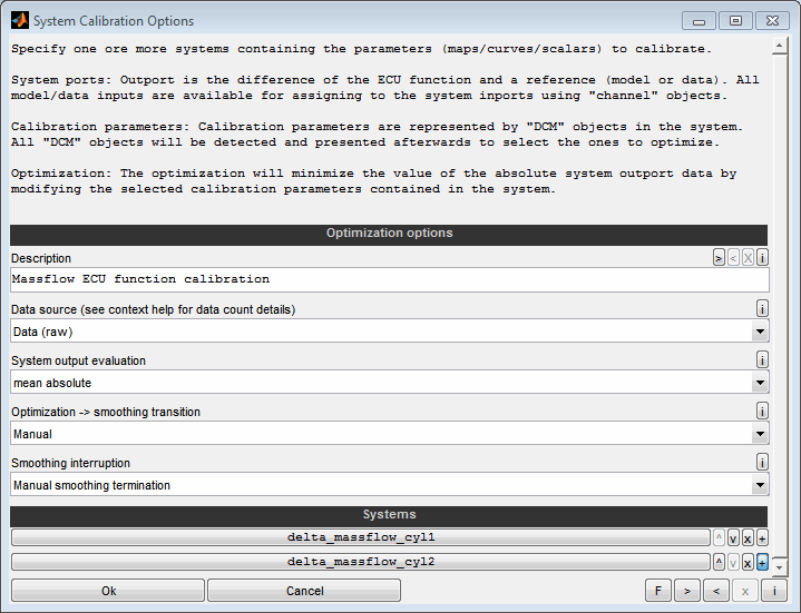
Description
You can enter a description to document and identify this system optimization during optimization and in the resulting files. This is especially helpful if multiple optimizations will be run in parallel.
Data source
Select where to retrieve the data accessible in the systems from. For details regarding the data count numbers of the single data sources see the help of the list dialogue field accessible by its context menu.
Data (raw)
The loaded data points will be considered for the calibration system optimization. The model itself (if any) remain unconsidered. Therefore no undesirable effects from the models in interpolated and extrapolated sections will occur but on the other hand the optimization will not benefit from the advantages of the models (data quality by the smoothness of the model and removed outliers).
Data (modeled)
The models will be interpolated at the input data values to generate the data for the optimization. Therefore the optimization will benefit from the advantages of the models (data quality by the smoothness of the model and removed outliers) but undesirable effects from the model in interpolated and extrapolated sections are eliminated.
If an output does not have a model, it is still available in the form of raw data so that it can be used as an auxiliary channel. In this way, channels can also be used that cannot be reasonably modeled - such as the time axis.
Model (entire)
The entire model data (axes grid points + output values) will be used for calibration system optimization.
Using the model includes the advantages in data quality by the smoothness of the model and removed outliers. But you need to check the plausibility of the result especially in extrapolated model sections. Outside the training data range or in sections with poor confidence the models may produce courses that look plausible but are impractical for the calibration system to reproduce. The optimization will then try to reduce the deviation in these areas at the expense of calibration quality inside the data ranges - this behavior is usually undesirable.
Model (confident part)
The confident part of the model (axes grid points + output values) will be used for calibration system optimization. The limit to judge a model to be confident can be edited using the “Edit model” feature.
This option maintains the advantages of the model (data quality by the smoothness of the model and removed outliers) and reduces the danger of unwanted behavior in extrapolated sections. The calibration will be optimized only based on model sections with known quality. However the models may still produce courses that are impractical for the calibration system to reproduce (e.g. in interpolated sections). The optimization will then try to reduce the deviation in these areas at the expense of calibration quality inside the data ranges - this behavior is usually undesirable.
System output evaluation
The optimization will always try to minimize a scalar rating value. You can select how to retrieve this scalar value from the system output that usually consists of multiple values because it will be calculated for all data source points.
The evaluation can be done by calculating the “mean absolute” or “maximum absolute” value. So for example if you choose “mean absolute” and the system output is the difference between an ECU function and its model representation, then the mean absolute difference for all data source points will be calculated.
You do not need to use abs() to calculate the absolute value of the system output to ensure meaningful error plots. This will be done automatically during optimization. The evaluation method will also be used to bring together the output of the single systems in case multiple systems were assigned.
So in our example the optimization will try to minimize the mean value of the two mean values of the two system outputs.
Optimization → smoothing transition
A system optimization consists of an optimization phase first followed by a smoothing phase. Both phases may be time consuming. To enable automatic usage e.g. overnight you can select an automatic transition from optimization to smoothing depending on a time or progress based criterion. Note that progress is often not linear. Even low rel. progress at the end of the optimization significantly improves the results from the point of view of the calibration engineer. Therefore, it makes sense to run the optimization until the result is plausible and completed by means of the intermediate results and to use the automatic transition options with care.
Manual
No automatic transition. User must terminate optimization to start smoothing.
Predicted progress [%] > (e.g. > 99% optimization progress)
Transition will be done automatically when the predicted progress is 99%. The predicted progress judges the change of the system output. 100% means a steady optimization state.
Relative progress step within recent past (e.g. 0.1% optimization progress in last 5h)
Transition will be done automatically when withing the last 5 hours the relative progress was less than 0.1%. The relative progress judges the system output directly. 100% would mean a perfect result with zero value of the system output.
Max. optimization duration [h] > (e.g. > 1h optimization duration)
Transition will be done automatically after a fixed optimization time without regarding a progress criterion.
Skip optimization - smooth immediately
No optimization will be performed. The smoothing phase is started immediately. This can be used to just smooth an existing calibration with respect to the systems output.
Individual
Afterwards you will have the possibility to enter individual settings.
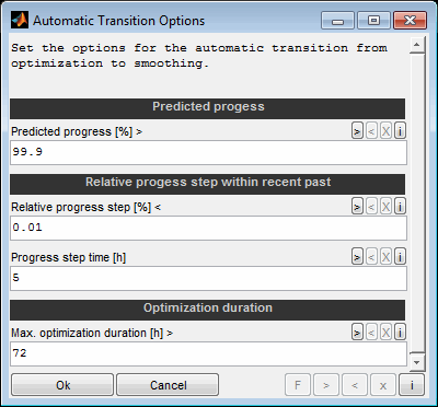
Smoothing interruption
The smoothing may be time consuming. To enable automatic usage e.g. overnight you can select an smoothing duration depending on a time or progress phase based criterion.
Specifying a maximum smoothing duration prevents the smoothing from continuing too far into areas with high errors during automated operation and then making mixing difficult at the end. This does not mean that the smoothing is finished. Only a dialog is displayed that allows you to exit. The smoothing can also be continued here.
Manual
No automatic interruption of the smoothing. User must terminate smoothing.
1..20 smoothing phases
Smoothing will be interrupted automatically after e.g. 20 smoothing phases. User can then decide to terminate or proceed smoothing.
1..72h smoothing duration
Smoothing will be interrupted automatically after e.g. 72 hours phases. User can then decide to terminate or proceed smoothing.
Systems
Specify one or more systems containing the parameters (scalars/curves/maps/3D+) to calibrate. The specification of the systems is done using the CalcGuide. Objects are available to integrate Simulink systems directly or by using a Host-Based Shared Library (*.dll).
System outport
Usually the output of a system is the difference of the ECU function output and the model output to indicate their deviation. You must not use abs() to calculate the absolute value. This will be done automatically during optimization. Otherwise the error plots available are meaningless.
System inports
All model inputs are available for assigning to the system inports using "channel" objects.
Calibration parameters
Calibration parameters are represented by "DCM" objects in the system. All "DCM" objects will be detected and presented afterwards to select the ones to optimize. Each “DCM” object must contain the parameter and file name. From the files the parameters will be loaded to retrieve the axes values and the initial values for the optimization.
Changed conventions for the dimensions must be observed. While in the SGE Circus, the x-axis is the horizontal axis of a map, in MATLAB/Simulink, for example, it is the vertical axis. Therefore, for direct use of the output of a DCM object as a Simulink block parameter, it is necessary to transpose. This is easy to achieve because it is an option of the DCM object.
It is essential to provide a plausible initial parameter calibration. Make sure to insert initial parameters into the calibration parameter file(s) with plausible range, shape and roughness.
To speed up the optimization or to exclude sections of the parameters from the optimization the parameters may contain NaN values. These values will be ignored during optimization. But make sure that the excluded sections do not influence the optimization result. Especially when parameters are sequentially integrated in calculations the values of one parameter will influence the inputs of the next one and therefore also its relevant section. As an example in the following figure the map MAP_LOAD will influence the significant section of the map MAP_IGNITION. Therefore for the map MAP_IGNITION NaN section must be used carefully.
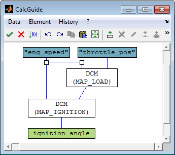
Intermediate signals
After system optimization, it will be possible to visualize the system outputs and the signals of the inputs before and after the optimization. This allows the detailed analysis of the result. In addition, there is the possibility to insert “Interim” objects into the calculation which makes these signals available for the analysis after optimization too. In this way also signals inside the calculation are accessible, e.g. the output of a Simulink simulation before application of differences and weightings.
Runtime performance
During the soptimization, the systems are executed very often. The duration of this calculation has a decisive influence on the overall system optimization. Therefore, using the configuation object in the CalcGuide, you should enable the option to optimize the runtime as soon as the systems expect to work properly. In the event of problems, the checks can be reactivated at any time.
Use the "systems duration" display available from the intermediate post processing to judge the runtime performance of the systems.
In general you should prefer manual mode first to be able to make the transition decision based on intermediate results. Additionally only manual transition makes available all post processing options. Automatic transitions set the post processing options automatically.
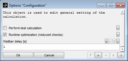
The following figure shows the implementation of the ECU system for cylinder 1 – first with the CalcGuide representation of the ECU function and then with an integrated Simulink system. See the CalcGuide documentation for details regarding the Simulink integration.
The output is the difference of the ECU function and the corresponding model output. Additionally big deviations are amplified keeping the sign.
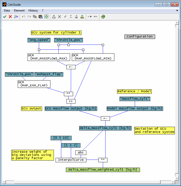
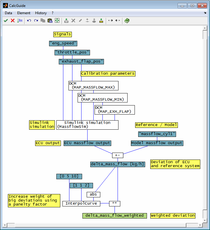
After detection of all calibration parameters inside the systems a list is presented to ask some more options. For optimization success it is essential to provide a plausible initial parameter calibration. Make sure to insert initial parameters into the calibration parameter file(s) with plausible range, shape and roughness. To speed up the optimization or to exclude sections of the parameters from the optimization the parameters may contain NaN values. These values will be ignored during optimization.
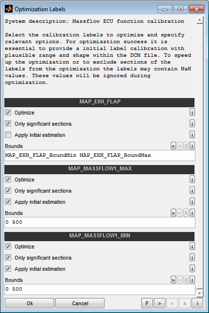
Optimize
Select whether to optimize the calibration parameter or to leave unchanged. For our example we choose to optimize all calibration parameters. In case the systems contain already calibrated parameters uncheck this option.
Only significant parameter sections
By default the entire parameter with all breakpoints will be optimized. But sometimes only part of the parameter is relevant when for example the measured or modeled data does not cover the entire parameter axes. If this option is enabled sections of the parameters not influencing the optimization result will be detected automatically in an initial test and removed from the optimization. This may be done to speed up the optimization.
Note that the type of calculation influences the result of the detection. Insignificant sections can be detected incorrectly if the calculation path is inactive. If, for example, two parameters are multiplied, one of which is zero in the initial dataset, then the other is incorrectly recognized as not significant, since a change in its values has no effect. The option "Only significant sections" may therefore only be used if the type of calculation and the initial date ensure that parameter changes are effective.
Remember that the test for relevance of the parameter sections is only done initially for the initial calibration. When the relevant parameter sections will change during optimization you must not enable this option because the optimization result will not cover all relevant sections or even may be wrong for the processed sections. Especially when parameters are sequentially integrated into calculations the values of one parameter will influence the inputs of the next one and therefore also its relevant section. As an example in the following figure the map MAP_LOAD will influence the significant section of the map MAP_IGNITION. Therefore “Optimize only significant parameter sections” must not be used for the map MAP_IGNITION.
Apply initial estimation
This option is used to create an initial estimation of the calibration parameter at the beginning of the optimization by quickly but roughly adjusting its course. Afterwards the optimization will finely tune the parameters. Usually this will result in an considerable speed up of the entire optimization.
Use this option if you expect a relevant change of the calibration parameter by the optimization. If the parameter already has a good initial calibration and the optimization is likely to change little, you should disable this option. Depending on the quality of the initial calibration it may happen that the relative progress at the beginning is temporarily negative when activating the initial estimation option.
The initial estimation progress could be inspected during intermediate post processing and should be 100% before the optimization is regarded as meaningful.
Bounds
Enter the sounds separated by spaces. Bounds can be defined in different ways.
Scalar values
limit the entire parameter to a single maximum and/or minimum value.
are defined by entering numerical scalar values.
Scalar offset values
limit the parameter to its initial value shifted by an offset.
the offset can be absolute or relative (by appending a %).
are defined by entering numerical scalar values surrounded by +()
allow a freely definable limitation.
must be located in the same calibration parameter file that contains the parameter to be calibrated.
are defined by their name inside the calibration parameter file.
will be interpolated to the axes of the parameter to calibrate using clipping outside the axes ranges. There are only monitored at at the axes breakpoints of the parameters to calibrate – not at the axes breakpoints of the bounds. Deviations from the bounds may occur in the intermediate areas.
Parameters from file
Bounds are also used to achieve a reproducible result for under-determined functions. This need exists when calibration parameters are summed up or multiplied and an infinite number of combinations exists that provide the same result. So when for example to calibration parameters to optimize are multiplied bounds must be applied to fix at least one single breakpoint value of of one of these parameters to ensure a reproducible result.
Make sure to only separate the lower and upper bound definition by spaces but not to use spaces inside the bounds definitions itself.
Examples:
"0 100" -> Lower limit 0, upper limit 100.
"+(-2) +(5%)" -> Lower limit initial - 2, upper limit initial +5%.
"Map_BoundMin Map_BoundMax" -> Lower limit defined by DCM parameter "Map_BoundMin", upper limit by parameter "Map_BoundMax".
"0 Map_BoundMax" -> Definition types can be mixed.
After entering all options some plausibility checks will be done and corresponding warning messages may be displayed. This is true when calibration parameters selected for optimization do have nearly no influence to the optimization result. Several reasons can cause this behavior:
Swapped or wrong input signals may cause a parameter to be interpolated always at the same breakpoints.
Parameters are limited by the bounds setting.
The initial calibration of one parameter deactivates the account of another parameter (e.g. by switches in the calculation).
Anyway this is only a hint and does not necessarily mean that a fault is present. Decide for yourself whether the behavior is desired and terminate the optimization if you want to change the settings.
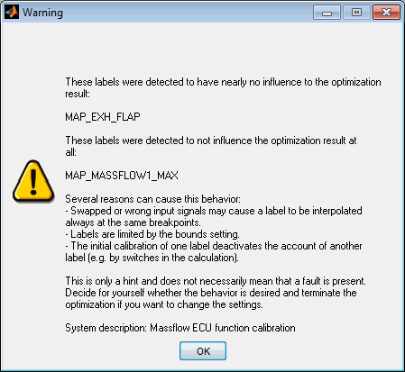
7.2.2 Optimization
In general the optimization is a two step procedure. First the actual optimization is done. Afterwards a smoothing step (post processing) is done to retrieve plausible and smooth calibration parameters.
The optimization will minimize the value of the absolute system outport data by modifying the selected calibration parameters. The “System output evaluation” setting determines how to retrieve a scalar value from the outport data.
In case multiple systems are specified their resulting values will be merged using the same evaluation as for the single systems (mean, maximum, minimum). So in our example the optimization will try to minimize the mean value of the two mean values of the two system outputs.
During optimization a progress bar is shown indicating the actual optimization state and the progress for some periods in the past. Using the “Options” button or closing the progress bar enables to terminate the optimization, to view and save intermediate results or to reconfigure the optimization settings. Some post processing options are already available from the waitbar directly using keyboard shortcuts (Status: Ctrl + a, Progress course: Ctrl + p, System signal visualization: Ctrl + i, Save calibration parameter file: Ctrl + s).
The post processing to access the intermediate results is explained in the following section.
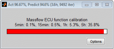
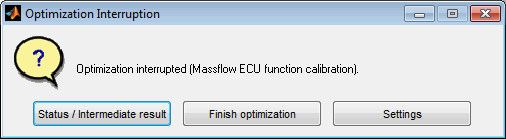
7.2.3 Post processing
The post processing enables to obtain plausible results from the raw mathematical optimization result which may be mendable in terms of plausibility and smoothness. Visualization, evaluation and smoothing routines support this post processing. It can be carried out as an interim result during optimization and as a final result after optimization.
Before starting the post processing all systems are evaluated once with the current best optimization result. So when an integrated Simulink system is used you can explore the simulation output (e.g. scopes, MATLAB workspace...) after starting post processing to judge the result.
Post processing options
The post processing options available differ when executed during or after optimization because some options are only available during optimization. For example as an intermediate result only some calibration parameters may be selected while as the final result all parameters will be selected automatically.
The following figures show the post processing options during (left) and after (right) optimization.
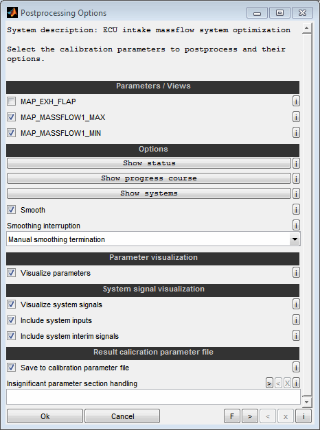
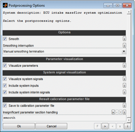
Parameters / Views
Select the calibration parameters to include into the post processing. As an intermediate result only some calibration parameters may be selected while as the final result all parameters will be selected automatically.
Show status
Some status information is available during optimization to assist judging the progress and to adjust settings if necessary. The status can also be accessed without interrupting the optimization by using the keyboard shortcut Ctrl + a when the waitbar is active.
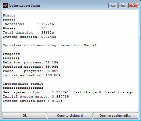
Show status
The "systems duration" is the current time spent to evaluate all systems once and might help to judge its performance.
Show progress course
The relative progress judges the system output directly. 100% would mean a perfect result with zero value of the system output. Especially when activating the initial estimation, the relative progress at the beginning can temporarily be negative.
The predicted progress judges the change of the system output. 100% means a steady optimization progress.
Especially when smoothness priority settings are activated it is worthwhile to invest sufficient time for the optimization as often progress regarding smoothness is reached at the end of the optimization.
The progress can also be accessed without interrupting the optimization by using the keyboard shortcut Ctrl+p when the waitbar is active.
Show systems
Use to display the systems to optimize. This is just a visualization and does not offer to edit the systems during optimization.
Intermediate result
The intermediate result is the minimum scalar rating value that occurred during optimization. The scalar rating value is calculated from the system output using the “System output evaluation” setting. It can be used to judge the status of the optimization and to detect mis-configuration of the system when implausible dimensions are noticed. The “systems invalid part" indicates the percentage of invalid (NaN) data of the systems output.
Show progress course
The progress course history since optimization start can be visualized graphically to judge the optimization status and to decide when to terminate the optimization.
The progress course can also be accessed without interrupting the optimization by using the keyboard shortcut Ctrl + p when the waitbar is active.
Relative optimization progress
The relative progress judges the system output directly. 100% would mean a perfect result with zero value of the system output. Especially when activating the initial estimation, the relative progress at the beginning can temporarily be negative.
Predicted optimization progress
The predicted progress judges the change of the system output. 100% means a steady optimization state.
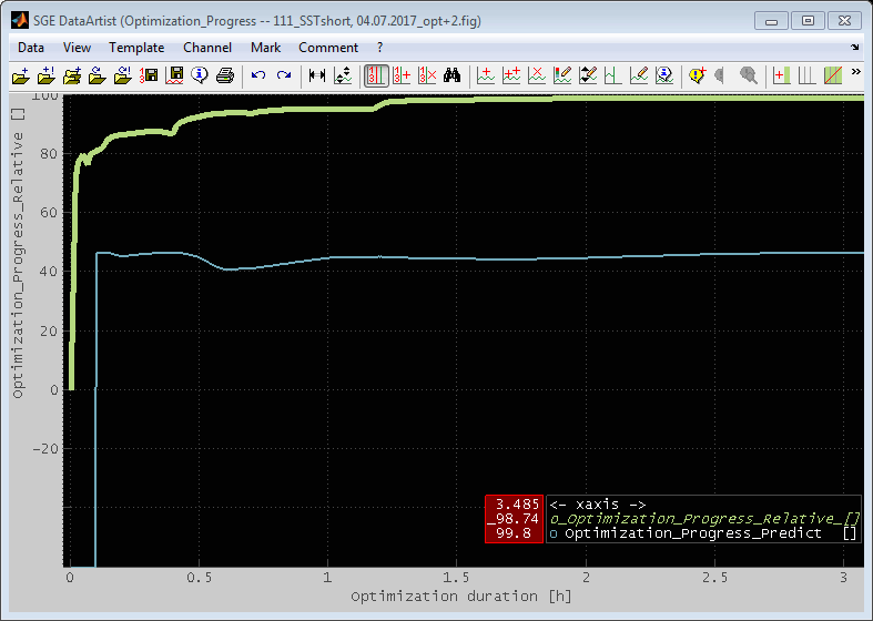
Smooth
The smoothing during post processing is a highly recommended option to obtain plausible results from the raw mathematical optimization result which may be amendable in terms of plausibility and smoothness. If selected, the parameters are smoothed automatically. This is accompanied by an elaborate graphical representation of the parameters, which also allows manual judgment and processing.
For the final post processing smoothing in mandatory and cannot be deselected.
See “Smoothing the optimization result” to understand how to use this for generating plausible and smooth results.
Smoothing interruption
Manual
No automatic interruption of the smoothing. User must terminate smoothing.
1..20 smoothing phases
Smoothing will be interrupted automatically after e.g. 20 smoothing phases. User can then decide to terminate or proceed smoothing.
1..72h smoothing duration
Smoothing will be interrupted automatically after e.g. 72 hours phases. User can then decide to terminate or proceed smoothing.
The smoothing may be time consuming. To enable automatic usage e.g. overnight you can select an smoothing duration depending on a time or progress phase based criterion.
Specifying a maximum smoothing duration prevents the smoothing from continuing too far into areas with high errors during automated operation and then making mixing difficult at the end. This does not mean that the smoothing is finished. Only a dialog is displayed that allows you to exit. The smoothing can also be continued here.
Visualize parameters
Using this option will visualize the selected parameters. During post processing after optimization all parameters will be visualized if this option is selected. Visualization is not supported for calibration parameters with more than two dimensions(3D+).
The system signals can also be accessed without interrupting the optimization by using the keyboard shortcut Ctrl + i when the waitbar is active.
In case of a map also data points will be transferred to the MapArtist (only when not using Simulink system integration). By this means the MapArtist enables some additional post processing of the resulting calibration parameters. Visualization will be done for the optimization result, the initial calibration, the raw optimization result before smoothing (if any) as well as for the result list resulting from the saved smoothing mixer states (if any).
The following figure shows the resulting map MAP_EXH_FLAP.
Visualize system signals
The course of the system outputs and all data channels can be visualized, which may be either inputs, outputs or intermediate results of the calculation.
Inputs and outputs will be visualized by default. In addition, there is the possibility to insert "Interim" objects into the calculation which make these signals available for the analysis too. This way also signals in the middle of the calculation are accessible, e.g. the output of a Simulink simulation before application of differences and weightings. Visualization will be done for the optimization result output, the initial calibration, the raw optimization result before smoothing (if any) as well as for the result list resulting from the saved smoothing mixer states (if any).
Use the subsequent options to specify the signals to include in detail.
See “System signals visualization” to understand how to use this for detailed optimization result analysis.
Save to calibration parameter file
If enabled the parameters will be saved to a calibration parameter file. If the result of the optimization is not satisfying the DCM saved may be used as initial values for a next optimization loop.
Some more information regarding optimization configuration, progress and result will also be saved to the calibration parameter file. See the comment of the single parameters regarding their meaning. So initial values, bounds, the optimization result before smoothing, the mean system outputs based on the calibration parameters inputs will be made available. When during smoothing additional states were saved these will also be saved.
A file can also be saved without interrupting the optimization by using the keyboard shortcut Ctrl + s when the waitbar is active.
Insignificant parameter section handling
The insignificant sections are displayed invisibly during optimization. To store in a calibration parameter file, all values of the parameters must be numeric. Decide how the insignificant sections are saved in a calibration parameter file.
Empty: If the field remains empty, the insignificant areas in the calibration parameter file are set to the initial calibration.
“smooth”: If you specify "smooth", the areas are additionally smoothed, if the smoothing is activated.
Numeric: If you specify a scalar numeric value, this is used for the ranges.
“NaN”: You can also specify "NaN" to maintain the insignificant sections for use in the SGE Circus. Note, however, that invalid values in calibration parameter files are not standard and that the files can not be read by other tools.
This setting does only apply to parameters with the “Only significant parameter sections” setting active.
7.2.4 Smoothing the optimization result
The smoothing during post processing is a highly recommended option to obtain plausible results from the raw mathematical optimization result which may be amendable in terms of plausibility and smoothness. If selected, the parameters are smoothed automatically. This is accompanied by an elaborate graphical representation of the parameters, which also allows manual judgment and editing of the parameters.
The smoothing algorithm does not perform the smoothing on its own. The quality is always taken into account by means of the system outputs. Also during manual editing you will always have the option to visualize and judge the effects of the work done considering the systems output. This is a major advantage compared to all later post processing.
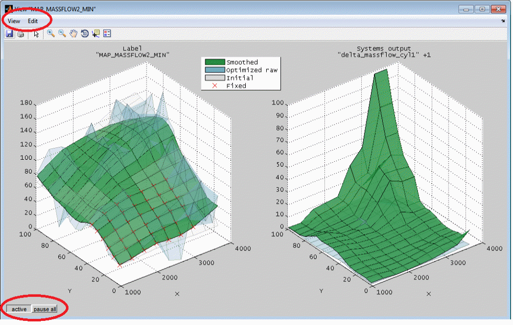
During smoothing progress windows are displayed separately for the single calibration parameters which are maps or curves. They are split into two sections. The left sections shows the actual parameter shape at the actual smoothing progress in addition to the initial shape and the raw optimized shape before smoothing start. The right section uses the same axes to visualize the system outputs. For each parameter breakpoint all relevant systems output values are calculated to a mean absolute value. The view for the system outputs is updated automatically during smoothing periodically. During mixing these views will be hided when parameters are set to inactive or edited manually. You need to update them manually using the corresponding menu or context menu item.
So the left section enables to judge the smoothness progress while the right section simultaneously enables to judge the resulting effect regarding the system outputs and therefore the optimization target.
The following options are available to influence the post processing:
“Active” status
Each progress window has a button to disable the smoothing for the individual parameters separately at sufficient progress. Disabling will also turn of the update of the right section and hide the display for the smoothed calibration parameter. When disabled the parameter will no longer be modified automatically.
Pause all
Each progress window has a button to pause the entire smoothing. This helps to find time for a thorough assessment of the status and manual actions like editing or freezing sections. During pause the view of the system output will still get refreshed to visualize e.g. effects of manual changes.
“Edit” menu
You can use this menu to influence the smoothing process. It is possible to manually adjust the parameter before or during smoothing as well as to freeze sections that are considered to be sufficiently smooth. To do this, the parameter is opened in the MapArtist. While the MapArtist is opened the automatic smoothing of the parameters is paused. To proceed and accept the manual changes terminate the MapArtist.
Edit manually
You can adjust the values of the calibration parameter manually. This can be helpful to support automatic smoothing in areas where experience has shown that shapes with increased errors can be drawn which the optimization does not find.
To edit the calibration parameter manually, use the MapArtist. There are then a large number of different possibilities for editing and smoothing. During manual editing it is not allowed to change the frozen or insignificant sections (= invalid) of the calibration parameter. Use the corresponding menu item to do this.
Freeze / unfreeze sections
The smoothness of a map often does not develop uniformly during automatic smoothing. Some areas sometimes require a lot of smoothing phases, while other areas are sufficiently smooth at an early stage. To avoid creating any unnecessary errors in these areas and still get the entire map smooth, it is possible to freeze sections of the map. These are then no longer changed by automatic smoothing. The frozen areas are highlighted in the graphic with markers.
To freeze areas, set them to invalid in the MapArtist. To reactivate frozen sections set then to a valid numeric value. During freezing/unfreezing changes of the values of the calibration parameter will be ignored. Use the corresponding menu item to do this.
“View” menu
The menu allows you to quickly adapt the display to your needs. It is possible to deactivate the automatic axis adaptation and arrange the active windows according to different criteria.
During smoothing a waitbar is visible to present the actual progress and the phase number. The smoothing process may consist of multiple phases. Smoothness will increase with ascending phase number as well as the system output values and therefore the loss of optimization target. The transition to the next phase is done automatically. When a quick increase in smoothness is desired a premature transition to the next phase can be forced using the “Intensify smoothing” option presented after pressing the “Options” button or closing the waitbar.
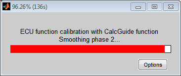
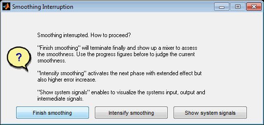
When the progress windows indicate a sufficient condition smoothing can be terminated also by closing the waitbar and choosing “Finish smoothing”. Afterwards post processing will proceed with an assisted consolidation – called mixing. See the following section for details.
Smoothing is not supported for calibration parameters with more than 2 dimensions (3D+).
7.2.5 Mixing the optimization result
The last result of smoothing is not always the optimal one with regard to all criteria. The smoothing may have run too long and caused increased errors. Or the assessment is not the same for all parameters. Some of them may be too smooth, others are not yet smooth enough. Therefore the final best result can now be put together individually, since after smoothing a large number of variations of the parameters are available, which differ in terms of plausibility, smoothness and errors. These are generated by the phases of automatic smoothing, manual changes during smoothing and freezing of parts of the parameters.
A smoothing mixer will show up and enables to balance the smoothing result between the initial state before smoothing and this set of parameter variations. All progress windows will update dynamically when moving the mixers slider. In this way, the entire smoothing process can be followed in detail and the decision can be made at which point the optimum result is achieved in every respect.
In addition to the system output visualization for every calibration parameter, the system signals visualization is also available to support the decision at any mixer state which enables to judge the inputs, outputs or intermediate results of the calculations for the current smoothing mixer state – see “System signals visualization” for details.
The view for the system outputs will be hided when parameters are set to inactive or edited manually because it cannot be generated from a saved state and needs to be recalculated. Therefore you need to update them manually using the corresponding menu or context menu item.
If no satisfactory state can be found in this way, there are additional options to create any combination of parameters that are not linked by the single mixer state.
Edit manually
It is possible to edit the parameters manually – just like it is done during smoothing. To do this, use the corresponding menu item and remember that you have to mark the parameters to edit as inactive, otherwise the changes will be lost. To edit the calibration parameter manually, use the MapArtist.
Individual “active” state
Additionally during mixing the “active” buttons of the single calibration parameters can be used to freeze the single parameters at different progress stages and create any combination of parameters independent from the mixer state. At the beginning of the mixing all deactivated parameters will be activated automatically.
Freeze / unfreeze sections
Similar to the proceeding during smoothing it is possible to freeze sections of the map. These are then no longer changed when the mixer is moved. The frozen areas are highlighted in the graphic with markers. At the beginning of the mixing all frozen section will be reset automatically.
To freeze areas, set them to invalid in the MapArtist. To reactivate frozen sections set then to a valid numeric value. During freezing/unfreezing changes of the values of the calibration parameter will be ignored. Use the corresponding menu item to do this.
The final slider state before closing the mixer window defines the smoothing state that will be used for further post processing – e.g. for visualization and saving to file.
Additionally an arbitrary number of additional mixer states can be added to a result list and also restored from the list. The corresponding parameters will also be available as a result in the visualization and saved files. The states can be given names and can be deleted individually.
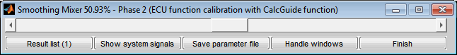
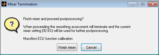
7.2.6 System signals visualization
The evaluation of the result of the optimization is supported by the visualization of various signals, which are either inputs, outputs or intermediate results of the calculation. All signals are made available for the states before optimization, after optimization before and after smoothing as well as all mixer states. The System signals visualization is available from post processing during and after optimization as well as during smoothing and mixing. Quick access is available using the shortcut Ctrl + i from the waitbar during optimization and smoothing.
Inputs and outputs will be visualized by default. In addition, there is the possibility to insert “Interim” objects into the calculation which make these signals available for the analysis after optimization too. This way also signals in the middle of the calculation are accessible, e.g. the output of a Simulink simulation before application of differences and weightings.
The following figure shows an example of a system and the visualization of its inputs, outputs and the Interim signals “ECU massflow output” and “Model massflow output”.
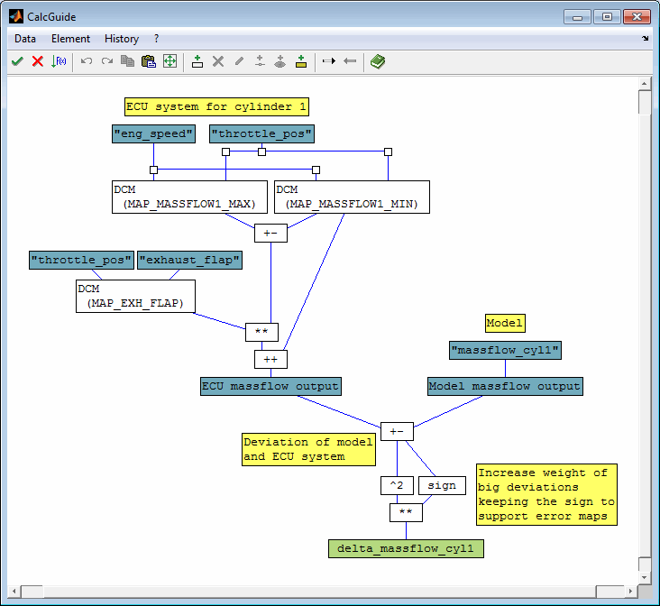
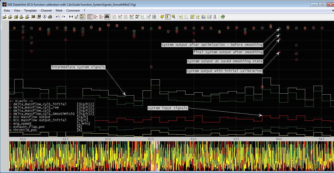
If the result of the optimization is not satisfying the resulting DCM may be used as initial values for a next optimization loop. A typical proceeding would look like this:
Start 1. optimization loop for all relevant parameters. Judge the progress and result by requesting intermediate results, apply smoothing and inspecting the “System signal visualization”.
Save the result and post process (smooth) some parameters that have a known shape.
Start 2. optimization loop with reduced parameter number to optimize. The result from the first loop is used as initial calibration and the post processed parameters will be deselected from optimization.
Again inspect the optimization progress and terminate if satisfying.
Save the result and post process (smooth) the remaining parameters.
7.3 Mark optimum
You can quickly set the cursors to an extreme of one output channel. You can select to use the data points or the model values (if any) and if you are interested in the maximum or minimum value.
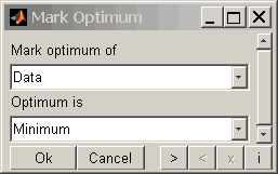
After the cursors were positioned at the optimum the resulting input and output values are displayed.
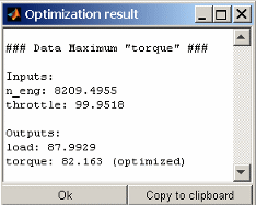
8 Save data
8.1 Save session
The whole session including data can be stored as file (Ctrl + Shift + s). After re-opening the whole functionality can be used again immediately.
Session files can be opened the same way as data files or using the SGE Viewer. Session files may get very large as they contain the loaded data.
9 Design of Experiment (DoE)
The SGE DoEArtist enables to create and visualize statistical test designs (DoE). Please see the corresponding documentation for further information.
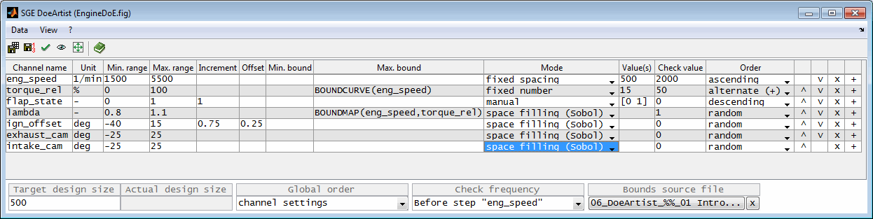
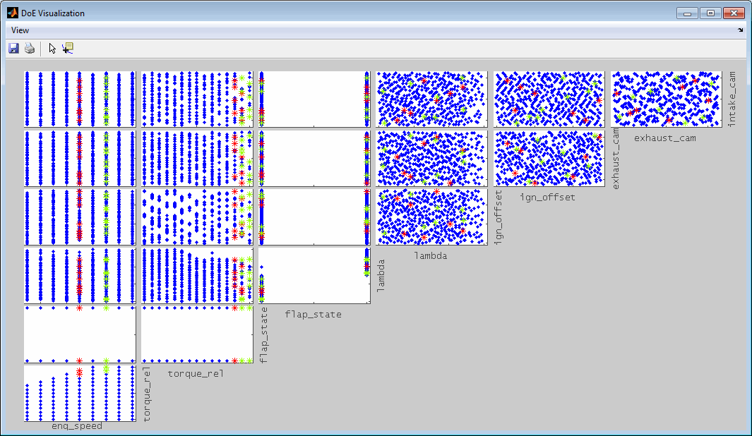
10 Present, print data
To be able to use the data and model also for presentation purposes, the ModelArtist makes it available to export the actual view into clipboard or file formatted in a way that is suitable to be useful for different targets (Ctrl + shift + c).
Document
Email
File
Printer
This can be different sizes of clipboard content. "Email" and "Document" are specially sized to fit into a email or document software. Some paper formats are also available and all windows can be printed and saved to various file formats.
The created plot is configurable. So you can move elements like legend or cursor boxes. It is also possible to add lines, arrows, text boxes etc. to the plot to explain or highlight.
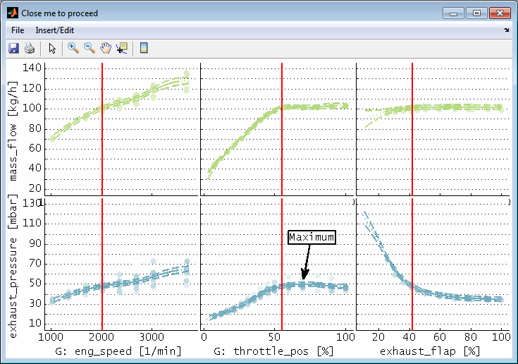
During creation some options will be asked to define the base layout of the plot.
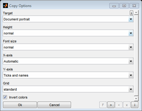
After closing the window the content will be copied to clipboard and can be pasted / used in the target software.
11 General information
Duplication, processing, distribution or any form of commercialization of the documents content beyond the scope of the copyright law shall require the prior written consent of the SGE Ingenieur GmbH. All trade and product names given in this document may also be legally protected even without special labeling (e.g. as a trademark).
MATLAB, Simulink and Stateflow are registered trademarks of The MathWorks Inc., Natick, MA, USA.
INCA is a registered trademark of ETAS GmbH, Stuttgart.
The SGE Circus includes Third Party Software. For details please refer to the → SGE Circus documentation.
SGE Ingenieur GmbH – www.sge-ing.de
Copyright 2011-